Multi-dividing Infinite Push Ontology Algorithm

(1)

Multi-dividing Infinite Push Ontology Algorithm

Wei Gao, Linli Zhu, and Yun Guo

Abstract_{—Along with the arrival of the era of large amount}

of data, many machine learning methods have been applied to the ontology similarity calculation and ontology mapping. In this paper, we raise an infinite push model for ontology similarity measuring and ontology mapping in multi-dividing setting. The iterative algorithm and generalization bound are given by virtue of the dual solution for optimization and the trick of covering number approach. Furthermore, the fast ontology algorithm for standard ontology SVM by virtue of infinite push multi-dividing ontology algorithm is obtained. Finally, four experiments presented on various fields verify the efficiency of the new computation model for ontology similarity measuring and ontology mapping applications in multi-dividing setting.

Index Terms_{—ontology, infinite push, similarity measure,}

ontology mapping, multi-dividing setting.

I. INTRODUCTION

T

HE term “ontology” is originally from the field of philosophy and it is used to describe the natural con-nection of things and the inherent hidden concon-nections of their components. In information and computer science, ontology is a model for knowledge storing and representation, and has been widely applied in knowledge management, machine learning, information systems, image retrieval, information retrieval search extension, collaboration and intelligent infor-mation integration. In the past decade, as an effective concept semantic model and a powerful analysis tool, ontology has been widely applied in pharmacology science, biology science, medical science, geographic information system and social sciences (for instance, see Przydzial et al., [1], Koehler et al., [2], Ivanovic and Budimac [3], Hristoskova et al., [4], and Kabir [5]).

The structure of ontology can be expressed as a simple graph. Each concept, object or element in ontology corre-sponds to a vertex and each (directed or undirected) edge on an ontology graph represents a relationship (or potential link) between two concepts (objects or elements). Let O be an ontology andGbe a simple graph correspond toG. The nature of ontology engineer application can be attributed to getting the similarity calculating function which is to compute the similarities between ontology vertices. These similarities represent the intrinsic link between vertices in ontology graph. The goal of ontology mapping is to get the ontology similarity measuring function by measuring the

Manuscript received March 31, 2015; revised May 12, 2015. This work was supported in part by the Key Laboratory of Educational Informatization for Nationalities, Ministry of Education, the National Natural Science Foundation of China (60903131), the College Natural Science Foundation of Jiangsu Province in China (10KJD520002) and the PhD initial funding of the first author.

W. Gao is with the School of Information and Technology, Yunnan Normal University, Kunming, 650500, China, e-mail: [email protected]. L. L. Zhu is with School of Computer Engineering, Jiangsu University of Technology, Changzhou, 213001, China, e-mail: [email protected].

Y. Guo is with School of Computer Science and Engineering, Soochow University, Suzhou 215006, China, e-mail: [email protected].

similarity between vertices from different ontologies. Such mapping is a bridge between different ontologies, and get a potential association between the objects or elements from different ontologies. Specifically, the ontology similarity functionSim:V ×V →R+∪ {0}is a semi-positive score function which maps each pair of vertices to a non-negative real number.

Very recently, ontology technologies have been employed in a variety of applications. Ma et al., [6] presented a graph derivation representation based technology for stable semantic measurement. Li et al., [7] raised an ontology representation method for online shopping customers knowl-edge in enterprise information. Santodomingo et al., [8] proposed an innovative ontology matching system that finds complex correspondences by processing expert knowledge from external domain ontologies and in terms of using novel matching tricks. Pizzuti et al., [9] described the main features of the food ontology and some examples of application for traceability purposes. Lasierra et al., [10] argued that ontologies can be used in designing an architecture for monitoring patients at home. More ontology applications on various engineering can refer to [11], [12] and [13].

The advanced idea to deal with the ontology similarity computation is using ontology learning algorithm which gets a ontology function f :V →R. By virtue of the ontology function, the ontology graph is mapped into a line which con-sists of real numbers. The similarity between two concepts then can be measured by comparing the difference between their corresponding real numbers. The essence of this idea is dimensionality reduction. In order to associate the ontology function with ontology application, for vertex v, we use a vector to express all its information. In order to facilitate the representation, we slightly confuse the notations and usevto denote both the ontology vertex and its corresponding vector. The vector is mapped to a real number by ontology function f : V →R, and the ontology function is a dimensionality reduction operator which maps multi-dimensional vectors into one dimensional vectors.

(2)

values of all classes are determined by experts. In this way, a vertex in a rate a has larger score than any vertex in rate b (if 1 ≤ a < b ≤ k) under the multi-dividing ontology functionf :V →R. Finally, the similarity between two ontology vertices corresponding to two concepts (or elements) is judged by the difference of two real numbers which they correspond to. Hence, the multi-dividing ontology setting is suitable to get a score ontology function for an ontology application if the ontology is drawn into a non-cycle structure.

In this article, we raise a new multi-dividing ontology learning algorithm for ontology similarity measuring and ontology mapping by means of infinite push. The rest of the paper is arranged as follows: in Section 2, the de-tailed description of infinite push multi-dividing ontology algorithms is showed, and the generalization bound is also yielded via covering number trick; in Section 3, we obtain the fast algorithm for ontology SVM training based on infinite push multi-dividing algorithm; in Section 4, four respective simulation experiments on plant science, humanoid robotics, biology and physics education are designed to test the efficiency of our infinite push based ontology algorithm, and the data results reveal that our algorithm has high precision ratio for these applications.

II. THEMULTI-DIVIDINGINFINITEPUSHONTOLOGY

ALGORITHM

Let V ⊂ Rd (d≥ 1) be a vertex space (or the instance space) for ontology graph, and the vertices (or, instances) in V are drawn randomly and independently according to some (unknown) distribution D. Given a training set S =

{v1,· · · , vn} of size n inV, the goal of ontology learning

algorithms is to obtain a score function f :V →R, which assigns a score to each vertex, and ranks all the instances according to their scores. The multi-dividing ontology prob-lem is a special kind of ontology learning probprob-lem in which vertices come from k categories and the learner is given examples of vertices labeled as therekrates.

Formally, the settings of multi-dividing ontology problems can be described as follows. There is an instance space V from which vertices are drawn, and the learner is given a training sample (S1, S2,· · ·, Sk) ∈ Vn1 ×Vn2 × · · · ×

Vnk _{consisting of a sequence of training sample} _S a = (va

1,· · ·, vnaa)(1≤a≤k). The goal is to learn from these

samples a real-valued ontology score function f : V → R that orders the future Sa vertices rank higher thanSb where

a < b. Hence, the empirical model for measuring the quality of ontology functionf can be expressed as

R(f;S) = k−1

X

a=1 k

X

b=a+1

max

1≤j≤nb

( 1

na na

X

i=1

I(f(via)< f(vbj))),

(1) where I(·) = 1 if the argument is held and 0 otherwise. The basic idea of (1) is to search an ontology function that guarantees the accuracy of top vertices for each rate a(1≤ a≤k). Such technology (concern the top vertices for each rate of the goal list) is called infinite push.

Since the function I(·) is non-differentiable, we should minimize (1) by using a continuous convex function instead of I. Specially, we consider the hinge ontology loss, which

forf, va_{, v}b _{is denoted as}

lH(f, va, vb) = (1−f(va−fb))+, (2)

whereu+ = max(u,0). Hence, we shall minimize a

regu-larized version of

RH₍_f_;_S_{) =} k−1

X

a=1 k

X

b=a+1

max

1≤j≤nb

( 1

na na

X

i=1

lH(f(vai)< f(vjb))),

(3) Let F be a real-valued ontology function space on V associated with a certain reproducing kernel. Let kfk_F be the RKHS norm off inF and the positive numberλbe a regularization parameter. Then the optimization problem can be stated as:

min f∈F[R

H₍_f_;_S_{) +}λ 2kfk

2

F]. (4)

In particular, we consider V =Rd andF as the class of ontology functionsf :Rd →Rwithf(v) =w·v for some w∈Rd. By usingkwk as the Euclideanl2 norm ofw and

employing w instead of f in RH₍_w_;_S₎_{, we infer that (3)}

becomes

min w∈Rd[R

H₍_w_;_S_{) +}λ 2kwk

2

F]. (5)

Conjunction with the definition ofRH₍_w_;_S₎_{, we deduce}

min w∈Rd[

λ

2kfk

2

F+

k−1

X

a=1 k

X

b=a+1

max

1≤j≤nb

( 1

na na

X

i=1

(1−w·(vai−vjb)))].

(6) For each pair of (a, b) (1 ≤ a < b ≤ k), let ξ_ija,b (1 ≤ i ≤ na,1 ≤ j ≤ nb) be the slack variables corresponding

to the max in the hinge loss terms (1−w·(va

i −vbj))+ =

max((1−w·(va

i −vbj),0). DenoteC= 1

λ, then (6) can be

re-written as

min w,ξa,b_ij

[λ 2kfk

2

F+C

k−1

X

a=1 k

X

b=a+1

max

1≤j≤nb

( 1

na na

X

i=1

ξa,b_ij )]

subject to ξ_ija,b≥1−w·(va

i −vbj) ∀i, j,(a, b)

ξ_ija,b≥0 ∀i, j,(a, b).

Moreover, by introducing further slack variablesξa,b

cor-responding to this max for each pair of (a, b), the above optimization model is transformed as

min w,ξa,b_,ξa,b

ij

[λ 2kfk

2

F+

k_X−1 a=1

k

X

b=a+1

C na

ξa,b]

subject to ξa,b_≥ na

X

i=1

ξ_ija,b, for j= 1,· · ·, nb

ξa,b_ij ≥1−w·(va

i −vjb) ∀i, j,(a, b)

ξ_ija,b≥0 ∀i, j,(a, b). (7)

In terms of Lagrange multipliers and the trick of dual, the optimization problem can be further re-written by variables {αa,b_ij : 1≤na,1≤j≤nb} for each pair of(a, b):

min αa,bij

[1 2

k−1

X

a=1 k

X

b=a+1

X

i,j

X

k,l

(3)

−

k_X−1 a=1

k

X

b=a+1

X

i,j

αij]

subject to nb

X

j=1

( max

1≤i≤na

αij)≤

C na

αa,b_ij ≥0 ∀i, j,(a, b). (8)

Let Qa,b₍_α₎ _{be the (quadratic) objective function in (8),}

and letΩa,b_⊆_Rmn_{be the feasible set for each pair of (}_{a, b}_),

i.e., the set ofαa,b_∈_Rnanb _{satisfying the constraints in (8).}

Then the projection algorithm starts with some initial value

(αa,b₎(1) _for _αa,b_{, and on each iteration} _t _{for special pair} (a, b), updates(αa,b₎(t)_{using a gradient and projection step:}

(αa,b)(t+1)← PΩa,b((αa,b)(t)−ηa,b_t ∇Qa,b((αa,b)(t))),

whereηa,bt >0 denotes a learning rate,∇Qa,b denotes the

gradient of Qa,b_{, and} _P

Ωa,b denotes Euclidean projection

ontoΩa,b_{. In the linear case, this gradient computation can}

be completed inO(dPk_a₌₁−1Pk_b₌_a₊₁nanb) time. Moreover,

it takes O(Pk_a−₌₁1Pk_b₌_a₊₁nanblog(nanb))time in the

pro-jection step. On solvingαa,b_{, the solution of (5) can be stated}

as

w= k−1

X

a=1 k

X

b=a+1

X

i,j

αa,b_ij (va i −vbj).

Returning to the general circumstances, V is any vertex space andF is an RKHS corresponding to a kernel function K:V×V →R. DenoteφK(x, y, z, u) =K(x, z)−Kx,u−

K(y, z) +K(y, u). By view of similar derivation, we derive the following kernel version of optimization problem:

min αa,bij

[1 2

k−1

X

a=1 k

X

b=a+1

X

i,j

X

k,l

αijαklφK(via, vbj, vka, vbl)

−

k_X−1 a=1

k

X

b=a+1

X

i,j

αij]

subject to k−1

X

a=1 k

X

b=a+1 nb

X

j=1

( max

1≤i≤na

αij)≤ k−1

X

a=1 k

X

b=a+1

C na

αa,b_ij ≥0 ∀i, j,(a, b). (9)

On solving αa,b _{for each pair of (}_{a, b}_{) (}₁_≤_{a < b}_≤_k_),

the solution to the original multi-dividing ontology problem is then obtained by

f(v) = k−1

X

a=1 k

X

b=a+1

X

i,j

αa,b_ij (K(va

i, v)−K(vbj, v)). (10)

Algorithm 1. Multi-dividing infinite push ontology algo-rithm:

Input: training sampleS= (S1, S2,· · · , Sk)∈Vn1×Vn2×

· · · ×Vnk _{and a kernel function}K:V ×V →_R

Fora= 1tok−1: Forb=a+ 1tok: Parameters Ca,b_{, t}a,b

max, η a,b 0

Initialize: α(1)_ij ← Ca,b

nanb ∀1≤i≤na,1≤j≤nb

For t = 1 to ta,b

max do: (αa,b) t+1

2 ← (αa,b)(t) −

η_√0a,b

t∇Q

a,b₍₍_αa,b₎(t)₎_,₍_αa,b₎(t+1)_{← P}

Ωa,b((αa,b)( t+1

2 )) End For.

End For. End For.

Output: f(v) = P_i,jα_ij(ta,b)∗(K(va

i, v)−K(vjb, v)), where (ta,b₎∗_{= argmin}

1≤t≤(ta,bmax+1)Q((αa,b) (t)₎_.

We emphasize here that the p-norm multi-dividing push ontology algorithm minimizes a convex upper bound on the lp-norm similar as the quantity in (1) for finitep:

Rp(f, S) = ( 1 nb nb X j=1 ( 1 na na X i=1

Π(f(via)< f(vbj)))p)

1

p. ₍₁₁₎

In the following part of the section, we give some theoreti-cal analysis for Algorithm 1. Assume vertices in ratea(here,

1≤a≤k) are drawn randomly and independently according to a distributionDa on V. LetD= (D1,D2,· · ·,Dk), and

define

R(f;D) = k−1

X

a=1 k

X

b=a+1

sup v∈supp(Db)

(Eva_∼D_a[I(f(v_ia)−f(v_jb))]),

(12) and

Ra,b₍_f_;_D_{) =} _sup v∈supp(Db)

(Eva_∼D a[I(f(v

a

i)−f(vbj))]), (13)

where supp(Db)denotes the support ofDb.

For anyγ >0, define the margin ontology loss as

lγ(f, vai, vjb) = I(f(vai)−f(vbj)≤γ),

and some notations are defined as follows:

Rγ₍_f_;_S_{) =} k−1

X

a=1 k

X

b=a+1

max

1≤j≤nb

( 1

na na

X

i=1

lγ(f, via, vbj)), (14)

Rγ₍_f_;_D₎ ₌ k−1

X

a=1 k

X

b=a+1

sup v∈supp(Db)

(Eva_∼D a[lγ(f(v

a i)

−f(vbj))]), (15)

Rγ,a,b₍_f_;_S_{) = max} 1≤j≤nb

( 1

na na

X

i=1

lγ(f, via, vbj)), (16)

Rγ,a,b₍_f_;_D₎ ₌ _sup v∈supp(Db)

(Eva_∼D a[lγ(f(v

a i)

−f(vb

j))]), (17)

lγ(f,Da, vb) =Eva_∼D_a[l_γ(f(v_ia)−f(v_jb))]. (18)

LetN(F, ε)be thel∞covering number ofF for radiusε,

i.e., the minimum number ofl∞balls with radiusεcoverF.

The generalization bound for the multi-dividing infinite push ontology algorithm is stated in the following conclusion. Theorem.LetFbe a class of real-valued ontology functions onV. Letε, γ >0, and

δa,b_D (f, γ, ε) =Pvb_∼D

b[lγ(f,Da, v

b₎_{< R}γ₍_f_;_D₎₋_ε_]_.

Then, we have

PS∼Dn1 1 ×D

n2

2 ×···×Dknk[∃f ∈ F:R γ₍_f_;_D₎

> Rγ₍_f_;_S_{) +}_ε_]

≤ N(F,εγ

8 ) k−1

X

a=1 k

X

b=a+1

(2nbe− na ε2

8

+(sup f∈F

(4)

Proof.The most important step in the proof is to bound the following probability

PS∼Dn1 1 ×D

n2 2 ×···×D

nk k [R

γ₍_f_;_D₎_{> R}γ₍_f_;_S_{) +}ε 2]

for given f ∈ F. On this purpose, we define

Rγ,a,b(f;Da, Sb) = max 1≤j≤nb

lγ(f,Da, vjb).

Then, we infer

PS∼Dn1 1 ×D

n2 2 ×···×D

nk k [R

γ₍_f_;_D₎₋_Rγ₍_f_;_S₎

> ε

2]

= PS[Rγ(f;D)− k−1

X

a=1 k

X

b=a+1

Rγ,a,b₍_f_;_D a, Sb)

+ k−1

X

a=1 k

X

b=a+1

Rγ,a,b(f;Da, Sb)−Rγ(f;S)>

ε

2]

≤

k−1

X

a=1 k

X

b=a+1

PSb[Rγ,a,b(f;D)−Rγ,a,b(f;D_a, S_b)

> ε

4] + k_X−1 a=1

k

X

b=a+1

PS[Rγ,a,b(f;Da, Sb)

−Rγ,a,b₍_f_;_S₎_> ε 4] = I+II.

We need to bound I andII. To boundII, we define

lγ(f, Sa, vb) = 1

na na

X

i=1

lγ(f, vai, vjb).

By Hoeffding’s inequality, we deduce

II =

k−1

X

a=1 k

X

b=a+1

PSa∪Sb[ max 1≤j≤nb

lγ(f,Da, vjb

− max

1≤j≤nb

lγ(f, Sa, vjb)>

ε

4]

≤

k−1

X

a=1 k

X

b=a+1

PSa∪Sb[ max 1≤j≤nb

|lγ(f,Da, vjb)

−lγ(f, Sa, vjb)|>

ε

4]

≤

k−1

X

a=1 k

X

b=a+1 nb

X

j=1

PSa∪Sb[|lγ(f,Da, v b j)

ε

4]

≤

k−1

X

a=1 k

X

b=a+1

nbsup vb

PSa[|l_γ(f,D_a, vb j)

ε

4]

≤

k−1

X

a=1 k

X

b=a+1

2nbe− na ε2

8 .

ForI, we yield

I =

k_X−1 a=1

k

X

b=a+1

PSb[sup vb

lγ(f,Da, vb)

− max

1≤j≤nb

lγ(f,Da, vjb)>

ε

4]

= k_X−1 a=1

k

X

b=a+1

PSb[ max 1≤j≤nb

lγ(f,Da, vjb)

<sup vb

lγ(f,Da, vb)−

ε

4]

= k_X−1 a=1

k

X

b=a+1

Πnb j=1Pvb

j[lγ(f,Da, v b j)

<sup vb

lγ(f,Da, vb)−

ε

4]

= k_X−1 a=1

k

X

b=a+1

(δ_Da,b(f, γ,ε

4)) nb_.

For any fixedf ∈ F, by combining I andII, we get

PS∼Dn1 1 ×D

n2 2 ×···×D

nk k [R

γ₍_f_;_D₎₋_Rγ₍_f_;_S₎_>ε 2]

≤

k_X−1 a=1

k

X

b=a+1

(2nbe− na ε2

8 + (sup

f∈F

δa,b_D (f, γ, ε/4))nb₎_.

The remaining proof from an application of standard tricks converts the above bound to a uniform convergence result that established uniformly over all f ∈ F using covering

number approach. ✷

III. FASTMULTI-DIVIDINGONTOLOGYALGORITHM FOR

ONTOLOGYSVM

The aim of this section is to present a fast training algorithm for standard multi-dividing ontology SVM by means of the same infinite push framework showed in the above section. The multi-dividing ontology SVM algorithm minimizes a regularized bound in (11) with p= 1over an RKHSF can be expressed as:

min f∈F[R

H

1(f;S) +

λ

2kfk

2

F], (19)

whereRH

1 (f;S) is defined in (11) with p= 1 and we use

hinge loss lH(f, vai, vbj) to replace the I(f(via) < f(vjb))

terms. By expanding (19) in terms of the definition of RH

1 (f;S), we get

min f∈F[

λ

2kfk

2

F+

k−1

X

a=1 k

X

b=a+1

1

Pk−1 a=1

Pk

b=a+1nanb na X i=1 nb X j=1 (1

−(f(va

i)−f(vjb)))+]. (20)

By introducing slack variables ξ_ija,b for each pair of (a, b)

corresponding to the max in the hinge loss terms (1 −

(f(va

i)−f(vjb)))+= max(1−(f(vai)−f(vjb)),0)and setting

C=_λ1, we obtain

min f,ξa,b ij

[λ 2kfk

2

F+

1

Pk−1 a=1

Pk

b=a+1nanb na X i=1 nb X j=1

ξa,b_ij ]

subject to ξ_ija,b≥1−(f(va

(5)

ξ_ija,b≥0 ∀i, j,(a, b).

By means of Lagrange multipliers and the dual technology, we get the following optimization problem in the nanb

variables {αa,b_ij : 1 ≤ i ≤ na,1 ≤ j ≤ nb} for each pair

of (a, b):

min αa,b_ij

[1 2

k−1

X

a=1 k

X

b=a+1

X

i,j

X

k,l

αijαklφK(via, vbj, vka, vbl)

−

k_X−1 a=1

k

X

b=a+1

X

i,j

αij]

subject to 0≤

k_X−1 a=1

k

X

b=a+1

αij ≤ k−1

X

a=1 k

X

b=a+1

C nanb

,

∀i, j,(a, b).

Algorithm 2.Fast multi-dividing training ontology algo-rithm via projection method

Inputs: training sampleS= (S1, S2,· · ·, Sk)∈Vn1×Vn2×

· · · ×Vnk _{and a kernel function}_K_:_V _×_V _→_R

Fora= 1tok−1: Forb=a+ 1tok: Parameters Ca,b_{, t}a,b

max, η a,b 0

Initialize: (αa,b_ij )(1) _← Ca,b

nanb ∀1≤i≤na,1≤j≤

nb

For t = 1 to ta,b

max do: (αa,b) t+1

2 ← (αa,b)(t) −

η_√0a,b

t∇Q

a,b₍₍_αa,b₎(t)₎

For1≤i≤na,1≤j≤nb:

If((αa,b_ij )(t+1

2 )<0) Then(αa,b

ij )(t+1)←0

Else if ((αa,b_ij )(t+1 2 )> C

a,b

nanb)Then(α a,b

ij )(t+1)← C a,b

nanb

Else _nCa,b

anb ←(α a,b ij )(

t+1 2 ) End For.

End For. End For. End For.

Output: f(v) = P_i,j(αa,b_ij )t∗ (K(va

i, v)−K(vbj, v)), where (ta,b₎∗_{= argmin}

1≤t≤(ta,bmax+1)Q

a,b₍₍_αa,b₎(t)₎_.

IV. EXPERIMENTS

The above ontology learning algorithms can be used in on-tology concepts similarity measurement and onon-tology map-ping. The basic idea is: via the ontology gradient computation model, the ontology graph is mapped into a real line con-sisting of real numbers. The similarity between two concepts then can be measured by comparing the difference between their corresponding real numbers. To show the effectiveness of our new ontology algorithms, four experiments concerning ontology measure and ontology mapping are designed below.

A. Ontology similarity measure experiment on plant data In the first experiment, we use plant “PO” ontology O1 which was constructed in the website

www.plantontology.org. The structure ofO1 is presented in

Fig. 1. P@N (Precision Ratio see Craswell and Hawking [17] is used to measure the quality of the experiment data.

We first give the closest N concepts for every vertex on the ontology graph by experts in plant field, and then we obtain the first N concepts for every vertex on ontology

graph by the algorithm 1 and 2, and compute the precision ratio. Specifically, for vertexvand given integerN >0. Let SimN,expert

v be the set of vertices determined by experts and

it containsN vertices having the most similarity ofv. Let

v_v1= argmin v′_∈_V₍_G₎₋_v

{|f(v)−f(v′)|},

v_v2= argmin v′_∈_V₍_G₎_−{_v,v1

v}

{|f(v)−f(v′)|}, · · ·

vN

v = argmin

v′_∈_V₍_G₎_−{_v,v1

v,···,v N−1

v }

{|f(v)−f(v′)|},

and

SimN,v algorithm={v1v, vv2,· · ·, vvN}.

Then the precision ratio for vertexv is denoted by

PreN v =

|SimN,algorithm

v ∩SimN,v expert|

N .

The P@N average precision ratio for ontology graph Gis then stated as

PreNG =

P

v∈V(G)Pre N v

|V(G)| .

At the same time, we apply ontology methods in [14], [15] and [16] to the “PO” ontology. Then we calculate the average precision ratio by these three algorithms and compare the results with algorithm 1 and algorithm 2 in the paper. Part of the data refer to Table 1.

When N= 3, 5 or 10, the precision ratio by means of our algorithms are higher than the precision ratio determined by algorithms proposed in [14], [15] and [16]. In particular, whenNincreases, such precision ratios are increasing appar-ent. Hence, the algorithms described in our paper are superior to the method proposed by [14], [15] and [16].

B. Ontology mapping experiment on humanoid robotics data

For the second experiment, we use “humanoid robotics” ontologies O2 and O3. The structure of O2 and O3 are

showed in Fig. 2 and Fig. 3, respectively. The ontology O2 presents the leg joint structure of bionic walking device

for six-legged robot, while the ontology O3 presents the

exoskeleton frame of a robot with wearable and power-assisted lower extremities.

The goal of this experiment is to give ontology mapping betweenO2 andO3. We also use P@N Precision Ratio to

measure the quality of experiment. Again, we apply ontology algorithms in [18], [15] and [16] on “humanoid robotics” ontology, and compare the precision ratio which are gotten from three methods. Some results refer to Tab. 2.

(6)

Fig. 1. The Structure of “PO” Ontology.

TABLE I

TAB. 1.THEEXPERIMENTRESULTS OFONTOLOGYSIMILARITY MEASURE

P@3 average P@5 average P@10 average

precision ratio precision ratio precision ratio

Algorithm 1 in our paper 0.5103 0.6176 0.7904

Algorithm in [14] 0.4549 0.5117 0.5859

Algorithm in [15] 0.4282 0.4849 0.5632

Algorithm in [16] 0.4831 0.5635 0.6871

TABLE II

TAB. 2. THEEXPERIMENTRESULTS OFONTOLOGYMAPPING

Algorithm in [18] 0.2778 0.4815 0.5444

Algorithm in [15] 0.2222 0.4074 0.4889

Algorithm in [16] 0.2778 0.4630 0.5333

Fig. 2. ‘Humanoid Robotics” OntologyO2.

(7)

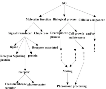
Fig. 4. The Structure of “GO” Ontology.

C. Ontology similarity measure experiment on biology data In the third experiment, we use gene “GO” ontology O4 which was constructed in the website

http: //www. geneontology. The structure ofO4is presented

in Fig. 4. Again, P@N is used to measure the quality of the experiment data. At the same time, we apply ontology method in [15], [16] and [19] to the “GO” ontology. Calculating the average precision ratio by these three algorithms and comparing the results to algorithm 1 and algorithm 2 rose in our paper, part of the data refer to Table 3.

When N= 3, 5 or 10, the precision ratio by virtue of our ontology algorithms are higher than the precision ratio determined by algorithms proposed in [15], [16] and [19]. In particular, when N increases, such precision ratios are increasing apparent. Therefore, the algorithms described in our paper are superior to the methods proposed by [15], [16] and [19].

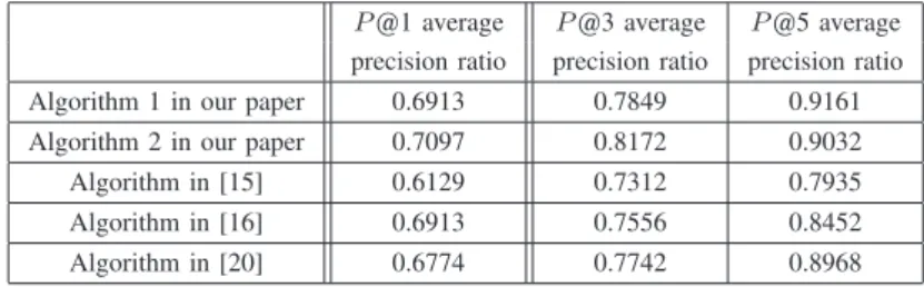
D. Ontology mapping experiment on physics education data For the last experiment, we use “physics education” on-tologiesO5 andO6. The structure ofO5andO6are showed

in Fig. 5 and Fig. 6, respectively.

The goal of this experiment is to give ontology mapping between O5 andO6. We also use P@N precision ratio to

measure the quality of experiment. Again, we apply ontology algorithms in [15], [16] and [20] on “physics education” ontology, and compare the precision ratio which is gotten from three methods. Some results refer to Tab. 4.

Taking N= 1, 3 or 5, the precision ratio in terms of our infinite push based ontology mapping algorithms are higher than the precision ratio determined by algorithms proposed in [15], [16] and [20]. Specially, as N increases, the precision ratios in view of our algorithms are increasing apparently. Therefore, the algorithms described in our paper are superior to the methods proposed by [15], [16] and [20].

V. CONCLUSIONS

As a data structural representation and storage model, ontology has been widely used in various fields and proved to

Fig. 5. “Physics Education” OntologyO5.

Fig. 6. “Physics Education” OntologyO6.

have high efficiency. One ontology learning trick is mapping each vertex to a real number, and the similarity is judged by the difference between the real number which the vertices correspond to. In this paper, we raise a infinite push learning model for ontology application in multi-dividing setting. The generalization bound is given by means of covering number approach. The experiments show the effectiveness of the new multi-dividing ontology algorithms. The new technology contributes to the state of art for applications and the result got in our paper illustrates the promising application prospects for multi-dividing ontology algorithm.

REFERENCES

[1] J. M. Przydzial, B. Bhhatarai, and A. Koleti, “GPCR Ontology: De-velopment and Application of AGProtein-Coupled Receptor Pharma-cology Knowledge Framework,”Bioinformatics, vol. 29, no. 24, pp. 3211-3219, 2013.

[2] S. Koehler, S. C. Doelken, and C. J. Mungall, “The Human Phenotype Ontology Project: Linking Molecular Biology and Disease Through Phenotype Data,”Nucleic Acids Research, vol. 42, no. D1, pp. 966-974, 2014.

(8)

TABLE III

TAB. 3. THEEXPERIMENTRESULTS OFONTOLOGYSIMILARITY MEASURE

P@3 average P@5 average P@10 average P@20 average

precision ratio precision ratio precision ratio precision ratio

Algorithm 1 in our paper 0.5171 0.6421 0.7942 0.9054

Algorithm 2 in our paper 0.5093 0.6401 0.7718 0.8653

Algorithm in [15] 0.4638 0.5348 0.6234 0.7459

Algorithm in [16] 0.4356 0.4938 0.5647 0.7194

Algorithm in [19] 0.4213 0.5183 0.6019 0.7239

TABLE IV

TAB. 4. THEEXPERIMENTRESULTS OFONTOLOGYMAPPING

Algorithm in [15] 0.6129 0.7312 0.7935

Algorithm in [16] 0.6913 0.7556 0.8452

Algorithm in [20] 0.6774 0.7742 0.8968

[4] A. Hristoskova, V. Sakkalis, and G. Zacharioudakis, “Ontology-Driven Monitoring of Patient’s Vital Signs Enabling Personalized Medical Detection and Alert,”Sensors, vol. 14, no. 1, pp. 1598-1628, 2014. [5] M. A. Kabir, J. Han, and J. Yu, “User-Centric Social Context

In-formation Management: An Ontology-Based Approach and Platform,”

Personal and Ubiquitous Computing, vol. 18, no. 5, pp. 1061-1083, 2014.

[6] Y. L. Ma, L. Liu, K. Lu, B. H. Jin, and X. J. Liu, “A Graph Derivation Based Approach for Measuring and Comparing Structural Semantics of Ontologies,”IEEE Transactions on Knowledge and Data Engineering, vol. 26, no. 5, pp. 1039-1052, 2014.

[7] Z. Li, H. S. Guo, Y. S. Yuan, and L. B. Sun, “Ontology Representation of Online Shopping Customers Knowledge in Enterprise Information,”

Applied Mechanics and Materials, vol. 483, pp. 603-606, 2014. [8] R. Santodomingo, S. Rohjans, M. Uslar, J. A. Rodriguez-Mondejar, and

M.A. Sanz-Bobi, “Ontology Matching System for Future Energy Smart Grids,”Engineering Applications of Artificial Intelligence, vol. 32, pp. 242-257, 2014.

[9] T. Pizzuti, G. Mirabelli, M. A. Sanz-Bobi, and F. Gomez-Gonzalez, “Food Track & Trace Ontology for Helping the Food Traceability Control,”Journal of Food Engineering, vol. 120, no. 1, pp. 17-30, 2014. [10] N. Lasierra, A. Alesanco, and J. Garcia, “Designing An Architecture for Monitoring Patients at Home: Ontologies and Web Services for Clinical and Technical Management Integration,” IEEE Journal of Biomedical and Health Informatics, vol. 18, no. 3, pp. 896-906, 2014. [11] M. Tovar and D. Pinto, Azucena Montes, Gabriel Gonzalez, and Darnes Vilarino, “Identification of Ontological Relations in Domain Corpus Using Formal Concept Analysis,”Engineering Letters, vol. 23, no.2, pp. 72-76, 2015.

[12] V. Gopal and N. S. Gowri Ganesh, “Ontology Based Search Engine Enhancer,”IAENG International Journal of Computer Science, vol. 35, no. 3, pp. 413-420, 2008.

[13] W. Gao and L. Shi, “Szeged Related Indices of Unilateral Polyomino Chain and Unilateral Hexagonal Chain,”IAENG International Journal of Applied Mathematics, vol. 45, no.2, pp. 138-150, 2015.

[14] Y. Y. Wang, W. Gao, Y. G. Zhang and Y. Gao, “Ontology Similarity Computation Use Ranking Learning Method,”The 3rd International Conference on Computational Intelligence and Industrial Application, Wuhan, China, 2010, pp. 20–22.

[15] X. Huang, T. W. Xu, W. Gao and Z. Y. Jia, “Ontology Similarity Mea-sure and Ontology Mapping Via Fast Ranking Method,”International Journal of Applied Physics and Mathematics, vol. 1, no. 1, pp. 54-59, 2011.

[16] W. Gao and L. Liang, “Ontology Similarity Measure by Optimizing NDCG Measure and Application in Physics Education,”Future Commu-nication, Computing, Control and Management, vol. 142, pp. 415-421, 2011.

[17] N. Craswell and D. Hawking, “Overview of the TREC 2003 Web Track,” In proceedings of the Twelfth Text Retrieval Conference, Gaithersburg, Maryland, NIST Special Publication, 2003, pp. 78-92. [18] W. Gao and M. H. Lan, “Ontology Mapping Algorithm Based on

Ranking Learning Method,” Microelectronics and Computer, vol. 28, no. 9, pp. 59-61, 2011.

[19] Y. Gao and W. Gao, “Ontology Similarity Measure and Ontology Mapping Via Learning Optimization Similarity Function,”International Journal of Machine Learning and Computing, vol. 2, no. 2, pp. 107-112, 2012.

[20] W. Gao, Y. Gao, and L. Liang, “Diffusion and Harmonic Analysis on Hypergraph and Application in Ontology Similarity Measure and On-tology Mapping,”Journal of Chemical and Pharmaceutical Research, vol. 5, no. 9, pp. 592-598, 2013.

W. Gao,male, was born in the city of Shaoxing, Zhejiang Province, China on Feb.13, 1981. He got two bachelor degrees on computer science from Zhejiang industrial university in 2004 and mathematics education from College of Zhejiang education in 2006. Then, he was enrolled in department of computer science and information technology, Yunnan normal university, and got Master degree there in 2009. In 2012, he got PhD degree in department of Mathematics, Soochow University, China.

Now, he acts as lecturer in the department of information, Yunnan Normal University. As a researcher in computer science and mathematics, his interests are covering two disciplines: Graph theory, Statistical learning theory, Information retrieval, and Artificial Intelligence.

L. L. Zhu, male, was born in the city of Badong, Hubei Province, China on Sep. 20, 1975. He got Master degrees on computer software and theory from Yunnan normal university in 2007. Now, he acts as associate professor in the department of computer engineering, Jiangsu University of Technology. As a researcher in computer science, his interests are covered two disciplines: computer network and artificial intelligence.