www.j-sens-sens-syst.net/3/105/2014/ doi:10.5194/jsss-3-105-2014
©Author(s) 2014. CC Attribution 3.0 License.
Open
Access
JSSS
Journal of Sensors and Sensor Systems
Principal component analysis for fast and automated
thermographic inspection of internal structures in
sandwich parts
D. Griefahn, J. Wollnack, and W. Hintze
Institute of Production Management and Technology (IPMT), TU Hamburg-Harburg, Denickestrasse 17, 21073 Hamburg, Germany
Correspondence to:D. Griefahn ([email protected])
Received: 15 August 2013 – Revised: 3 March 2014 – Accepted: 7 April 2014 – Published: 14 May 2014
Abstract. Rising demand and increasing cost pressure for lightweight materials – such as sandwich structures – drives the manufacturing industry to improve automation in production and quality inspection. Quality in-spection of honeycomb sandwich components with infrared (IR) thermography can be automated using image classification algorithms. This paper shows how principal component analysis (PCA) via singular value de-composition (SVD) is applied to compress data in an IR-video sequence in order to save processing time in the subsequent step of image classification. According to PCA theory, an orthogonal transformation can project data into a lower dimensional subspace with linearly uncorrelated principal components preserving all origi-nal information. The effect of data reduction is confirmed with experimental data from IR-video sequences
of simple square-pulsed thermal loadings on aramid honeycomb-sandwich components with CFRP/GFRP
(carbon-/glass-fiber-reinforced plastic) facings and GFRP inserts. Hence, processing time for image
classi-fication can be saved by reducing the dimension of information used by the classiclassi-fication algorithm without losing accuracy.
1 Introduction
Lightweight materials – such as sandwich structures – ex-perienced and are forecasted to see a rising demand due to overall increasing transportation volumes especially in avia-tion. Driven by fuel efficiency requirements, the higher share
of lightweight materials also in the traditional transportation industry will further augment this demand. This overall in-crease continuously drives the manufacturing industry to im-prove automation in production and quality inspection. To-day, sandwich is – thanks to its excellent combination of me-chanical strength but also damping properties and the low av-erage material density – a commonly used macro- and micro-composite construction. Sandwich components with carbon-or glass-fiber-reinfcarbon-orced plastic (CFRP/GFRP) facings are
typically deployed in rough environments with locally high loadings. In order to cope with heavy concentrated loads or to connect with other structures, components are designed with molded-in inserts, e.g., made from short glass
fiber-reinforced plastic. These inserts replace the honeycomb core to absorb stresses in a defined way (Bitzer, 1997). Quality in-spection requires controlling these inserts for presence, cor-rect type, and deviation of geometrical location inside the component after the fabrication step. Due to the mostly in-transparent sandwich facings, normal visual inspection meth-ods fail to perform the described tasks, whereas infrared (IR) thermography combined with image classification algo-rithms delivers promising results for facing thicknesses be-low half a millimeter.
Pulsed thermography methods are characterized by a shorter cycle time but lower depth resolution. Both are commonly used methods and established for the testing of small lots at laboratory level (Maldague, 2001; Ibarra-Castanedo et al., 2009).
This study evaluates the potential of the square-pulsed thermography for detection of macroscopic subsurface struc-tures in large sandwich components and shows an approach for automated inspection.
2 Background on principal component analysis and automated detection in IR sequences
As described, thermography is a very well investigated NDT (nondestructive testing) method with many different
techni-cal variants for the active testing approach (Maldague, 2001; Ibarra-Castanedo et al., 2009). All techniques aim at max-imizing contrast directly in the thermal image or to apply algorithms to create or improve contrast in a second step. Principal component thermography (PCT) is a computational approach for analyzing thermal material behavior over time (Rajic, 2002), further improvement can be obtained with con-trast enhancement methods and thermal behavior modeling (Omar et al., 2010; Feuillet et al., 2012). An automation of the qualitative PCT approach can be achieved by adding a supervised learning step for image classification (Marinetti et al., 2004).
2.1 Principal component analysis (PCA) using singular value decomposition (SVD)
Principal component analysis is a technique widely used in the context of machine vision (e.g., face recognition or re-mote sensing), but also for image and video compression. PCA applies a linear transformation to a group of correlated variables in such a way that the obtained set of transformed variables is uncorrelated (Jackson, 1991). The principal com-ponents are typically computed via a SVD.
In order to perform a PCA using SVD on infrared video se-quences (spatial temperature information over time) the 3-D thermographic data need to be rearranged into a 2-D matrix. Image information (nx-by-ny), wherenxandnyrepresent the number of photosensitive elements on the sensor in xand y direction, is reshaped into an nx·ny-by-1 matrix for ev-ery time step. This operation preserves the original spatial information of temperature on the specimen surface, since the reverse transformation is unique. The subsequent trans-formation of allnttime steps in the video sequence creates annx·ny-by-ntmatrixAin which time variations are stored column-wise and spatial variation row-wise.
According to the theory of SVD, any matrixX(P-by-Q, P≤Q) can be factorized as follows:
X=ΩΓVT, (1)
whereΩis aQ-by-Qmatrix,Γis aP-by-Qmatrix with
pos-itive or zero diagonal elements representing the singular val-ues andVTis the transposed of aP-by-Pmatrix. The
decom-position of IR-data in the matrixA(M-by-N,M = nx·nyand
N=ntand thereforeM >N) can be determined by comput-ing and decomposcomput-ingAATor using the “reduced” or
“econ-omy” SVD form to obtain
A=USVT, (2)
whereUis anM-by-Nmatrix containing spatial information
in the orthogonal space. Since spatial information inAare
arranged vertically, the columns of Urepresent a set of
or-thogonal statistical modes called empirical oror-thogonal func-tions (EOF) (Emery and Thomson, 2004). The rows ofVT
describe the characteristic time behavior of the correspond-ing orthogonal function – called principal component vectors building the principal component space. The vectors can pro-vide a measure for time behavior and characterize the defect depths in the material. The matrixSis anN-by-N diagonal
matrix with the singular valuessjof A. The principal com-ponents are obtained scaling the EOFs by multiplyingUwith Sor by projectingAvia a multiplication withVinto the
prin-cipal component space. It can be shown that
AAT=US2UT (3)
to derive that the singular valuessjare the square roots of the positive eigenvalues ofAAT, which is the co-variance matrix
ofAmultiplied with the factor (M−1). This relationship al-lows creating a relative measure for the share of cumulated variance included in the firstiEOFs.
νEOF(i)=
Pi j=1sj
Pnt j=1sj
i∈[1,nt] (4)
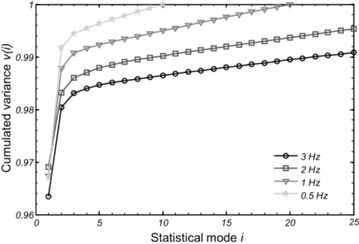
Earlier investigations state that more than 95 % of variance can be contained in the first three to five statistical modes and respective components (Marinetti et al., 2004).
2.2 Instance-based learning withk-nearest neighbor Instance-based learning is used for classification when an ex-plicit description of the target function is not available. The instance-based algorithms store training data for classifica-tion of future instances. Thek-nearest neighbor algorithm
is the most basic and very common kind of instance-based learning classifiers.
The k-nearest neighbor algorithm classifies points in an n-dimensional space based on the Euclidean distance to the k nearest points in the training sample. Depending on the
selection of k the classification result can differ (Mitchell,
c
Processing
5
Synchroni-zation
4
Time Loading
IR camera
1
Specimen
3
Halogen lamps
2
T(xi,yj)
th tc
dl
dm
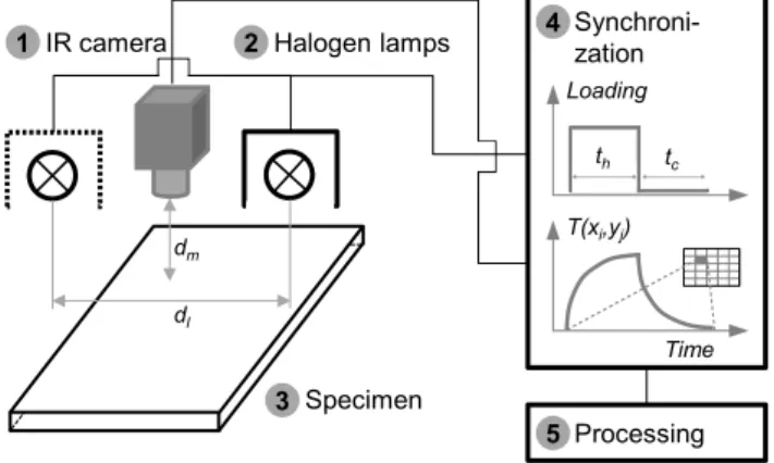
Figure 1.Test field for infrared inspection.
The approach for supervised learning on IR sequences is to generate sets of training data from EOFs with known geome-tries for different materials and corresponding test settings.
3 Experimental setup for square-pulsed thermographic inspection
The following section describes the experimental setup for the square-pulsed thermographic inspection including test field configuration, the deployed sandwich specimen, and the test settings
3.1 Test field configuration
Figure 1 shows the test field setup used for the described ex-periments. An IR camera (1) is installed equilaterally with two 400 W halogen lamps at a lateral distance ofdl=250 mm (2), which are used as heat sources. The halogen lamps as well as the IR camera have a distance ofdm=200 mm to the
tested sandwich specimen. The deployed IR camera is an Op-tris PI400 with sensor resolution of 382 pixels by 288 pixels, a thermal sensitivity of 80 mK, and maximum measurement frequency of 80 Hz. The halogen lamps are equipped with a reflector plate in order to homogenize the radiation on the specimen (3) surface. The camera captures the radiation emitted by the specimen’s surface.
The synchronization unit (4), which is also linked to the IR-camera recording software, triggers the halogen lamp via a relay and applies the thermal loading during the heating phase. The camera records the heating and the cooling phase. The algorithms for SVD and k-nearest neighbor described
in Sect. 2 subsequently perform the processing (5) using MATLAB (version 2012b). LabVIEW (version 2011) cou-pled with a digital I/O (input/output) device synchronizes the
measurements.
Sandwich construction Fabricated component
a b
Facing
Adhesive
Facing Core
Insert
Close-out
Figure 2.Schematic setup of sandwich structures with close-out
and inserts(a)and fabricated component(b) according to Bitzer (1997).
3.2 Tested specimens
Sandwich panels (Fig. 2) are generally built from a dense and strong facing, an adhesive layer and a core. The role of the adhesive layer is to bond the facing to the top and bottom sides of the lightweight core.
Facing material can be metallic such as steel, titanium or aluminum as well as nonmetallic material such as glass fiber, Kevlar-reinforced plastic or carbon-fiber-reinforced plastic. For composite materials such as prepregs, the matrix mate-rial may substitute the effect of the adhesive layer (Bitzer,
1997). The earliest core material used for aviation purposes was balsa wood after World War I, and is still in use for some applications. Mostly for nonaerospace applications, ex-panded polymer foams and aluminum foams can be found as core material today. Honeycomb cores clearly dominate all other cores in aerospace. Honeycomb core structures can be produced from almost all typical lightweight materials such as aluminum, regular, and reinforced polymers or paper. Aramid-fiber paper impregnated with phenolic resin is to-day’s most used honeycomb material (Karlsson and Åström, 1997).
Figure 2a additionally shows an example for a close-out and a high-strength insert element. Close-close-outs fulfill the function of mechanical protection of the component’s edges and a barrier for humidity penetration. Close-outs are added cofabricated during master shaping as polymer filling of the honeycombs as shown in Fig. 2 (Bitzer, 1997).
3.2.1 Sandwich panel fabrication
of less than 800 mm×800 mm, but only smaller sections are inspected.
3.2.2 Specimens material
All specimens used for the experiments are fabricated from typical aircraft-grade materials and produced under condi-tion of mass produccondi-tion for the aviacondi-tion industry.
For test purposes, two types of pressed honeycomb sand-wich modifications with intransparent facings have been se-lected – one with a CFRP-based facing and the other with a GFRP-based facing. The aramid honeycomb core used has a cell-size of 3.2 mm. The CFRP specimen, with a total thick-ness of 9.7 mm, is covered with a 0.5 mm facing based on woven carbon-fiber phenolic resin and bonded to the aramid honeycomb core. The GFRP specimen, with a total thick-ness of 15.5 mm, is composed of a 0.3 mm woven fiberglass facing with phenolic resin and also bonded to an aramid hon-eycomb. For in-service reasons, the GFRP sample is covered with a thin but intransparent polymer protection foil. Both are equipped with GFRP inserts and in the potting step lo-cally filled with thermoplastic polymer for edge close-out. The diameter of the inserts, locally replacing the honeycomb core of the specimens, is 18 mm for the CFRP specimen and 45 mm for the GFRP specimen. The dimensions of edge close-outs range from approximately 10 mm for the CFRP specimen to 20 mm for the GFRP specimen; given the accu-racy of the potting and the filling behavior of the honeycomb cells the width varies a few millimeters.
3.3 Test settings
Heating timeth and cooling timetc have to be selected de-pending on the material of the sandwich facing (see Sect. 4.1 for the exact settings) and the facing layer thickness. CFRP facings require increased heating time or higher power of halogen lamps. This is due to the high heat flow transversal to the test direction given the higher conductivity of carbon compared to glass fibers. The required spatial resolution for the purpose of quality assurance defines the distance between camera and specimen resulting from the field of view.
4 Experimental results
4.1 Contrast improvement via PCA
Video sequences are acquired with heating time th,GFRPand cooling timetc,GFRP, each of 10 s, on a GFRP sample result-ing in a sequence lengthtm,GFRPof 20 s for the total measure-ment. The CFRP sample was tested at a heating timeth,CFRP and cooling timetc,CFRP, each of 20 s, resulting in a sequence lengthtm,CFRPof 40 s for the total measurement. In order to investigate the influence of the amount of provided input data on the PCA, measurement frequency fm is varied with the steps 0.5, 1, 2, and 3 Hz. The number of resulting images or
0 5 10 15 20
0.96 0.97 0.98 0.99 1
Statistical mode i
C
um
ul
at
ed v
ar
ianc
e v
(i
)
3 Hz 2 Hz 1 Hz 0.5 Hz
25
Statistical mode i
C
um
ul
at
ed v
ar
ianc
e
v
(i
)
Figure 3.Cumulated and normalized varianceνEOF for the first
25 statistical modes.
dimensionntof the matrixAis given by the following equa-tion:
nt=(th+tc)·fm=tm·fm. (5) Figure 3 shows the normalized varianceνEOF cumulated in the firstiso-called statistical modes and corresponding EOFs
for the GFRP sample. According to Eq. (3), this measure cumulates the firsti singular values in S corresponding to
the firstispatial components or EOFs in columns of the
ma-trixU. The value is normalized with the total variance.
The first dimension of the video matrixAcontains the total
number ofnx·ny=382·288=110 016 elements. At the max-imum frequency of 3 Hz and the given recording time, the number of time steps and second dimensionnt of the video matrixAequals to 60 elements.
The analysis shows that the relatively slow process of heat conduction through materials with partially very low ther-mal conductivity does not require measurement frequencies above 1 Hz to cover more than 99 % of the time behavior of sandwich material in the first three EOFs. At minimum, the Shannon theorem in the time domain must be fulfilled.
For a measurement frequency of 1 Hz raw, thermal data without emissivity correction are shown on a grayscale in Fig. 4 (GFRP specimen (a) and CFRP specimen (b)) for three selected and representative instances. The first image of the heating phase as well as the first and the last image of the cooling phase are displayed. The SVD is performed in a sub-sequent step to obtain the EOFs from the thermal data.
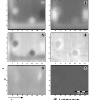
Figures 5 and 6 show the effect of decreasing variance on
the specimen with GFRP and CFRP facings respectively. It visualizes that the information from an IR-video sequence of square-pulsed thermal images are compressed into three to four EOFs. The retransformation of the columns of matrix
Uas described in Sect. 2.1 delivers the spatial information
50 100 150 200 250 300 350 50
100
150
200
250
50 100 150 200 250 300 350
50
100
150
200
250
50 100 150 200 250 300 350
50
100
150
200
250
1
21
nt Time step
x
y 40
50 100 150 200 250 300 350
50
100
150
200
250
20
50 100 150 200 250 300 350
50
100
150
200
250
50 100 150 200 250 300 350
50
100
150
200
250
1
11 a b
50 mm 50 mm
Figure 4.Thermal images at the time stepsntfor the GFRP
spec-imen(a)and the CFRP specimen(b)(first image in heating, first and last image in cooling phase).
CFRP sample contains the direct reflections from the heat sources occurring at the shiny specimen surface.
This section demonstrated that PCA can be applied to square-pulsed thermography for inspection of sandwich components by delivering compressed spatial information with improved contrast between subsurface elements in sand-wich structures by preserving time-variation data.
4.2 Automated detection
The aim of the automated detection is to obtain segmented images for the purpose of further inspection. Thek-nearest
neighbor algorithm requires an amount of preclassified data. These so-called training data are generated from the sand-wich samples from known geometric locations (e.g., center of the insert or close-out, plain honeycomb) that are manu-ally classified.
Figure 7 visualized such set of training data for the first three EOFs of the GFRP specimen for approximately 5000 preclassified pixels, which are a subset in the dimensionM
(nx·ny). Each data point corresponds to the intensity values from the first three images in Fig. 5 for the same selected pixel. Thek-nearest neighbor algorithm uses the training data
to classify a “new” instance (in this case the nonclassified data from the sequence) of data – pixel by pixel – based on the Euclidian distance to thek-nearest neighbors. For the
ex-50 100 150 200 250 300 350
50
100
150
200
250
50 100 150 200 250 300 350
50
100
150
200
250
50 100 150 200 250 300 350
50
100
150
200
250
50 100 150 200 250 300 350
50
100
150
200
250
50 100 150 200 250 300 350
50
100
150
200
250
50 100 150 200 250 300 350
50
100
150
200
250
1 2
3 4
5 6
i Statistical mode i x
y
50 mm
Figure 5.First 6 EOFs of the GFRP specimen.
periments,kvaries from three to five depending on the other
test settings. In theory, the algorithm can perform the classi-fication tasks in real numbersRn, whereas onlyi=n
tfeatures for classification are available from the IR sequence. Based on the result that 99 % or more of the variance is retained in the first few EOFs, even a reduction of the dimension of the feature space has to be considered.
Two types of definitions for classification errors are used to assess the performance of the algorithm depending on the dimension of the feature space in terms of classification ac-curacy and computation speed. An algorithm implements the definitions to obtain repeatable and automated results. All inspected parts contain subsurface elements that can be as-sumed as closed contours on the level of pixel size. If all (or all but one) neighboring pixels in a classified image differ
from the class of the selected pixel, it is obviously falsely classified. Figure 8 illustrates the definition of classification errors type I and type II in a segmented image.
Figure 9 shows the results from the classification perfor-mance analysis. All data are normalized to 100 % for i=1
50 100 150 200 250 300 350 50 100 150 200 250
50 100 150 200 250 300 350
50
100
150
200
250
50 100 150 200 250 300 350
50
100
150
200
250
50 100 150 200 250 300 350
50
100
150
200
250
50 100 150 200 250 300 350
50
100
150
200
250
50 100 150 200 250 300 350
50
100
150
200
250
1 2
3 4
5 6
i Statistical mode i x
y
50 mm
Figure 6.First 6 EOFs of the CFRP specimen.
-3.4 -3.2 -3 -2.8 -2.6
-2.4 x 10⁻³
-10 -5
0 5
x 10-3
-0.025 -0.02 -0.015 -0.01 -0.005 0 0.005 0.01 0.015 EOF(1) EOF(2) E O F( 3 ) Insert Close-out Honeycomb EOF(1) EOF(2) E OF (3 )
Figure 7.Visualization of first three EOFs of the GFRP-training
sample.
the computation effort by a factor of 100, while significantly
increasing the computation effort, the classification accuracy
does not improve but worsens by 15 % for error type I. Using only the first EOF as feature space for thek-nearest neighbor
classification is comparable to applying a histogram-based approach with multiple thresholds. Feature space dimensions between two and five deliver up to 30 % improved results for classification accuracy regardless of the type of error def-inition and show the advantage of reduced ambiguity. Re-sults from Fig. 3 explain the described effect of falling
ac-curacy when adding statistical modes beyond the fifth one.
Close-out
Insert Honeycomb
Classified image Classification errors
Type I
Type II
Figure 8.Definition of detectable classification errors by type.
0 5 10 15
100 1.000 10.000
First i statistical modes used for classification
C om upat ion t im e
0 5 10 15 2050
100 150 200 N um ber of er ror s
Error type I Error type II Computation time (log)
All data normalized to 100 for i = 1
10,000
1,000
First i statistical modes used for classification
C om put at ion ti m e [ % ] N um ber of e rro rs [ % ]
All data normalized to 100 for i = 1
Figure 9.Normalized plot of computation time and number of
oc-curring errors for classification for the GFRP sample based on the firstistatistical modes.
Every additional mode contains only a very small amount of additional information useful for classification. It mostly increases noise in the image due to the high rate of data com-pression.
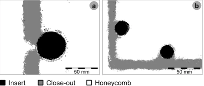
Figure 10 shows the final results for the classification of the GFRP specimen (a) and the CFRP specimen (b). The GFRP specimen – tested at the setting specified above – is processed using the three first EOFs and based on the three nearest neighbors relationship. Heating and cooling time for the CFRP sample are both increased by 5 s to obtain suf-ficient contrast. Processing requires including the first five EOFs and using the five nearest neighbors to improve classi-fication results. The color code in the images for the different
subsurface structures reflects the classification result. Both tests show that subsurface structures in sandwich compo-nents with fully intransparent facing materials are detectable. The images show a specimen of surface of approximately 100 cm2, which is tested in less than 30 s including process-ing time for classification. Decreasprocess-ing the spatial resolution by pixel in the test setup further improves this ratio.
5 Conclusions
Close-out Insert
a b
Honeycomb
50 mm 50 mm
Figure 10.Classification result for the GFRP specimen(a)and the
CFRP specimen(b).
instance-based classification algorithm detects and separates subsurface structures in sandwich components with intrans-parent facing material.
All investigations aimed at identifying suitable test set-tings to ensure fast and reliable results for the detection. The experiments confirm the effect of data reduction via PCA into
the first three to five statistical modes from previous investi-gations and suggest limiting the measurement frequency to avoid noise from oversampling of a slow thermal process. The numerical evaluation of the cumulated variance in the transformed sequences fortifies the result. Principal compo-nent thermography on sandwich compocompo-nents is a very robust technique to improve contrast on square-pulsed-tested IR se-quences and has a lower sensitivity to inhomogeneous light-ning than e.g., simple threshold methods in image process-ing.
The combination with the k-nearest neighbor algorithm
enhances the setup to a method for automated detection and classification of subsurface structures. Three to five statistical modes covering more than 99 % of variance deliver clearly an optimum result with respect to classification accuracy and a relatively low computation effort.
Future investigations focus on a prediction of thermal be-havior of sandwich material based on numerical simulations. This will help to improve the current set of training data in the transition between different subsurface structures and
will show approaches for automated population of training data.
Acknowledgements. The project on which this paper is based
was funded by the German Federal Ministry of Economics Affairs and Energy under funding code 20W1115C. The authors assume all responsibility for the content of this publication.
Edited by: R. Tutsch
Reviewed by: two anonymous referees
References
Bitzer, T.: Honeycomb technology: Materials, design, manufactur-ing, applications and testmanufactur-ing, 1st Edn., Chapman & Hall, London, 1997.
Emery, W. J. and Thomson, R. E.: Data analysis methods in physi-cal oceanography, 2. and rev. ed., 3. impr., Elsevier, Amsterdam, 2004.
Euro-Composites©, Infrastructure and production technologies
– Panel Production: http://www.euro-composites.com/en/ technology/Seiten/panel.html (last access: 13 March 2013), 2009.
Feuillet, V., Ibos, L., Fois, M., Dumoulin, J., and Candau, Y.: De-fect detection and characterization in composite materials using square pulse thermography coupled with singular value decom-position analysis and thermal quadrupole modeling, NDT&E Int., 51, 58–67, 2012.
Ibarra-Castanedo, C., Piau, J.-M., Guilbert, S., Avdelidis, N. P., Genest, M., Bendada, A., and Maldague, X. P. V.: Compara-tive Study of AcCompara-tive Thermography Techniques for the Nonde-structive Evaluation of Honeycomb Structures, Res. Nondestruct. Eval., 20, 1–31, 2009.
Jackson, J. E.: A user’s guide to principal components, Wiley series in probability and mathematical statistics, Wiley, 1991. Karlsson, K. F. and Åström, T. B.: Manufacturing and applications
of structural sandwich components, Compos. Part A-Appl. S., 28, 97–111, 1997.
Maldague, X. P. V.: Theory and practice of infrared technology for nondestructive testing, Wiley series in microwave and optical en-gineering, Wiley, New York, NY, 2001.
Marinetti, S., Grinzato, E., Bison, P. G., Bozzi, E., Chimenti, M., Pieri, G., and Salvetti, O.: Statistical analysis of IR thermo-graphic sequences by PCA, Infrared Phys. Techn., 46, 85–91, 2004.
Mitchell, T. M.: Machine learning, International ed., McGraw-Hill series in computer science, McGraw-Hill, New York, NY, 1997. Omar, M. A., Parvataneni, R., Zhou, Y.: A combined approach of self-referencing and Principle Component Thermography for transient, steady, and selective heating scenarios, Infrared Phys. Techn., 53, 358–362, 2010.