Trends in epidemiology in the 21st century:
time to adopt Bayesian methods
Tendências da epidemiologia no século XXI:
é o tempo dos métodos bayesianos
Tendencias de la epidemiología del siglo XXI:
es tiempo para los métodos bayesianos
1 Faculdade de Medicina de Ribeirão Preto, Universidade de São Paulo, Ribeirão Preto, Brasil.
Correspondence E. Z. Martinez
Faculdade de Medicina de Ribeirão Preto, Universidade de São Paulo.
Av. Bandeirantes 3900, Ribeirão Preto, SP 14049-900, Brasil. [email protected]
Edson Zangiacomi Martinez 1
Jorge Alberto Achcar 1
Abstract
2013 marked the 250th anniversary of the pre-sentation of Bayes’ theorem by the philosopher Richard Price. Thomas Bayes was a figure little known in his own time, but in the 20th century the theorem that bears his name became widely used in many fields of research. The Bayes theo-rem is the basis of the so-called Bayesian meth-ods, an approach to statistical inference that allows studies to incorporate prior knowledge about relevant data characteristics into statis-tical analysis. Nowadays, Bayesian methods are widely used in many different areas such as astronomy, economics, marketing, genetics, bioinformatics and social sciences. This study observed that a number of authors discussed re-cent advances in techniques and the advantages of Bayesian methods for the analysis of epide-miological data. This article presents an over-view of Bayesian methods, their application to epidemiological research and the main areas of epidemiology which should benefit from the use of Bayesian methods in coming years.
Bayes Theorem; Statistics; Probability Theory
Resumo
O ano de 2013 marca o 250o aniversário da
apresentação do teorema de Bayes pelo filósofo Richard Price à Royal Society em 1763. Thomas Bayes foi uma pessoa pouco conhecida em sua época, mas no século XX o teorema que leva o seu nome tornou-se amplamente utilizado em muitas áreas de pesquisa. O teorema de Bayes é a base dos chamados métodos bayesianos, um procedimento de inferência estatística que per-mite incorporar na análise o conhecimento pré-vio sobre características relevantes dos dados. Atualmente, os métodos bayesianos são larga-mente usados em muitas diferentes áreas como astronomia, economia, marketing, genética, bioinformática e ciências sociais. Em adição, é observado na literatura que muitos autores têm discutido os recentes avanços do uso dos méto-dos bayesianos na análise de daméto-dos epidemio-lógicos. No presente artigo, apresentamos uma visão global dos métodos bayesianos, sua utili-dade na pesquisa epidemiológica e os tópicos em epidemiologia em que estes métodos podem ser extensivamente usados nos próximos anos.
Introduction
The first mathematical formulation using the Bayesian method is attributed to Thomas Bayes, a British Presbyterian minister. Very little is known about his personal history. It is believed that he was born around 1701 in Hertfordshire, England and died in 1761 in Tunbridge. Many facts about his life are speculation such as the exact date of his birth and the authorship of a book on Theology entitled Divine Benevolence: or an Attempt to Prove That the Principal End of the Divine Providence and Government is the Hap-piness of His Creatures, that concerned the mo-tive behind God’s actions in making the world. In 1719, he began his studies of logic and theology at the University of Edinburgh. The only scientific work published during his lifetime was The Doc-trine of Fluxions, in 1736, in which he defended the logical foundation of Isaac Newton’s calculus. Two years after his death, his friend Richard Price (1723-1791) presented the Royal Society with a manuscript authored by Thomas Bayes entitled An Essay Towards Solving a Problem in the Doc-trine of Chances1. Price said he found the essay
among Bayes’ papers and in his opinion it “has great merit and well deserves to be preserved” 2
(p. 451). The essay offered the first clear solution to a problem of inverse probability, where Bayes described how we can calculate the probability of the occurrence of an event given the known probability of a certain condition. This formula is known as Bayes’ theorem. It is interesting to note that Richard Price believed that Bayes’ theorem was based on theological arguments and it could prove the existence of God 3. In 1748, the Scottish
empiricist philosopher David Hume published a book entitled An Enquiry Concerning Hu-man Understanding. In chapter ten of this work entitled Of Miracles, Hume wrote his famous argument against miracles 4. Today, some
au-thors claim that Hume’s statements were based on arguments taken from Bayes’s theorem 5,6,7.
Despite these philosophical ideas, Bayes’ essay seemed to have been forgotten until the publica-tion of the book entitled Théorie Analytique des Probabilités by the French mathematician and astronomer Pierre-Simon Laplace, in 1812. It is believed that Laplace was not familiar with the work of Thomas Bayes and he independently de-veloped a more formal version of Bayes’ theorem. Currently, Bayesian ideas are used in many fields of technology and research, such as mod-ern computers which use Bayesian filters to clas-sify emails and detect spam 8. Another example
of the modern use of Bayesian ideas is in robots which, based on a Bayesian framework 9 and a
Bayes network based system, distinguished
ter-restrial rocks from meteorites in the first robotic identification of a meteorite in 2000 in the El-ephant Moraine in the Antarctic 10. In addition,
NASA’s Mars Exploration Rover mission has been using Bayesian classification algorithms to study the physical properties of the surface of Mars 11.
Nowadays, Bayesian methods are widely used in many different fields of research, such as as-tronomy 12, economics and econometrics 13,14,
marketing 15, actuarial science 16, psychological
research 17, genetics 18,19, evolutionary biology 20,
bioinformatics 21, demography 22, social
scienc-es 23, public health 24, drug development 25 and
clinical trials 26,27. The use of Bayesian methods
in epidemiological studies has been discussed by several authors 28,29,30,31 and Congdon 32 claims
that the Bayesian approach is very useful for modeling epidemiological datasets, since they allow the control of possible confounding influ-ences on disease outcomes and the establish-ment of causal and dose-response relationships. In addition, Dunson 28 showed that the use of
Bayesian techniques in epidemiological studies is a powerful mechanism for incorporating in-formation from previous studies and controlling confounding. Appropriate methods for dealing with interactions between variables and con-founding effects are essential for epidemiologi-cal studies, and in this respect Bayesian methods can be very useful. Bayesian methods represent a totally different way of thinking about research methods where the researcher’s previous knowl-edge and experience have an important effect on inference and decision-making.
The traditional approach to statistical infer-ence is the frequentist (or classical) technique, where results are interpreted in terms of the fre-quency of occurrence of an event observed in a hypothetically large number of repetitions of the experiment. Frequentist inferences are based only on observational data, while Bayesian infer-ence assumes that prior knowledge can be for-mally incorporated into the analytical process. We can therefore say that the Bayesian research method is based both on an empirical world represented by the sample data and on human reasoning represented by the accumulated expe-rience of the researcher.
Are we in the Bayesian era?
In 1996, David Moore published an article 33
that discussed the possibility of teaching Bayes-ian inference on a first statistics course for stu-dents from different backgrounds. He argued that Bayesian methods were rarely used in prac-tice and teaching them would deprive students of instruction about more common statistical methods. It is possible that this statement was based on limitations caused by the time needed for software and hardware to analyze data using a Bayesian approach. Major advances in software and hardware in the last 20 years have been one of the factors that has led to a sharp increase in the use of Bayesian methods. To obtain an idea of the current use of Bayesian methods in health research, a search was made in PubMed using the keyword “Bayesian”. The annual number of articles is presented graphically in Figure 1 which shows that the first article using the term “Bayesian” indexed in PubMed was published in 1963 34. After this first publication, we observe a
very modest increase in the number of articles up to the middle of the 1980s, after which a large increase can be observed. It is important to re-member that portable personal computers on-ly became popular in the middle of the 1980s,
significantly contributing to the use of Bayesian methods, since the approach is usually depends on computational algorithms. A large increase in the number of published articles using the term Bayesian can be observed toward the end of 20th
century. It is possible that this increase was due to the emergence of new software adapted to Bayesian analysis, such as the free software Win-BUGS 35. This software uses simulation
meth-ods, such as the popular Markov Chain Monte Carlo (MCMC) methods 36, and was possibly the
most important computational advances to have popularized the use of Bayesian methodology. The first version of WinBUGS for Windows was made available in 1997 37. Today, OpenBUGS is
the open-source version of WinBUGS and can be freely downloaded from the project website (http://www.openbugs.info/w/Downloads).
In 2010, 2.56 in every 1,000 articles indexed in PubMed contained the term Bayesian (Fig-ure 1), showing the growing use of Bayesian methods in health research since the publica-tion of Moore’s article 29 and suggesting that
Bayesian statistics is actually an important is-sue to students who are starting their studies to become researchs. The advantages of the use of Bayesian methods in specific fields of knowl-edge, such as genetics 18, oncology 38 and
para-Figure 1
Results of the search of PubMed for articles containing the term Bayesian. The line shows the number of articles containing the term Bayesian published each year divided by the total number de articles indexed in that year (x 1,000).
2010 Year
1960 1970 1980 1990 2000
0.0 0.5 2.5
2.0
1.5
1.0
sitology 39, have therefore been discussed in
a number of research articles available in the literature.
One of the reasons for the widespread use of Bayesian methods may be related to the ease with which statistical inferences can be made even with complex problems. It is therefore expected that the use of Bayesian methods will continue to increase in response to the demands of ever more complex problems in the health field.
A practical example: estimating disease
prevalence
In order to illustrate Bayesian inference pro-cedures, let us consider a simple example in which we estimate the prevalence θ of a disease among the inhabitants of a given community. A parameter is defined as an unknown numeri-cal characteristic of a population. Prevalence θ is therefore a parameter and may be estimated using a frequentist or Bayesian approach. First, let us describe how this is done using the fre-quentist approach. A sample of size n is repre-sented by a probability function, defined as the likelihood function and denoted by f(x|θ). In the frequentist approach, inference is based only on the likelihood function. Xi is a random binary variable which assumes the value of 1 if the i -th individual has -the disease of interest and -the value of 0 if the i-th individual does not have the disease: (i = 1,…,n). Thus, the probability of the i-th individual having the disease is P(Xi = 1) = θ, and the probability of the individual not hav-ing the disease is P(Xi= 0) = 1 – θ, where 0≤θ≤1. In this case, we say that Xi follows a Bernoulli distribution with success probability θ, and its probability function is given by P(Xi = xi) = θ xi
(1 – θ)1 –xi, where x
i assumes the value 0 or 1. Assuming that X1, X2, …, Xn are independent random variables, that is, assuming that an individual having the disease does not affect the probability of another individual having the disease, the likelihood function is given by
The maximum-likelihood estimation (MLE) procedure is a frequentist method commonly used to estimate the parameters of a statistical model 40,41. Using the MLE method the estimate
of a parameter θ is given by the value of this pa-rameter in the papa-rameter space (set of all pos-sible values of the parameter) that maximizes the likelihood function f(x|θ). For this purpose, we can use differential calculus tools to obtain an es-timator ^ of θ. In practice, it is often more conve-nient to maximize the logarithm of the likelihood f(x ) = n P X( x )= n x(1 – )1 –x = (1 – )n– .
i =1 i i i =1 i i
= ∑ni=1xi ∑ni=1xi
function, also called the log-likelihood function. If we set the first derivative of the log-likelihood function equal to zero, the maximum likelihood estimator ^ of θ is given by
∑n n
number of individual with the disease in the sample total number of individuals in the sample
i=1xi
^
= =
This is a well-known expression which can be found in many widely used epidemiology text-books. Inference is then based on a hypothetical series of data sets collected under identical con-ditions. For example, a 95% confidence interval is a range of values calculated from the sample observations, with 95% certainty that all possible random samples drawn from the same popula-tion using the same sampling scheme would gen-erate intervals containing the true value of the parameter. However, a 95% confidence interval does not mean that there is a 95% probability that the calculated interval contains the true value of the parameter. Although this interpretation is quite intuitive, it is not valid since the frequentist method cannot assign probabilities to any par-ticular parameter.
The frequentist approach assumes that the parameter of interest is a fixed quantity, while in the Bayesian approach parameter uncertainty is represented by a probability distribution. From a statistical viewpoint, this is perhaps the most striking difference between the traditional fre-quentist approach and the Bayesian approach and is cause of much controversy, since frequen-tist stafrequen-tisticians do not accept the parameters to be represented by random variables.
In Bayesian analysis, a prior probability distribution for all parameters in the statistical model is necessary. On observing that the prev-alence of the disease is in a limited range (0,1), a plausible prior probability distribution is as-signed to a parameter θ given by a beta distribu-tion 42, a flexible probability distribution which
can take many forms depending on the values of a and b. In this case, the prior distribution f (θ) for θ has a probability density function given by
f 1 a– 1 b– 1, 0 < < 1,
=B a,b( ) (1 – )
( )
its standard deviation to one quarter of the dis-tance between the limits 2% and 30% (for further details see Browne 200143) thus giving a = 4.96
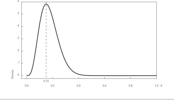
and b = 23.45. The graph in Figure 2 shows the probability density function of the beta distri-bution with parameter values of 4.96 and 23.45 mathematically representing the prior informa-tion given by the epidemiologist. It can be ob-served that the maximum value of the probability density function is 15% (the mode). In addition, it can be seen that the probability of prevalence be-ing higher than 30% or lower than 2% is low. This process is called prior probability elicitation 44.
The likelihood function plays a key role in sta-tistical inference in both frequentist and Bayes-ian approaches. The Bayes’ theorem says that the distribution of θ given the data (named pos-terior distribution) is proportional to the prod-uct of the prior distribution f (θ) and likelihood function f (x|θ). Bayes’ formula establishes that f(Ө|x) f(Ө)
x
f(x|Ө).Thus, we have f (x|θ) = k x θa+ ∑
n
i=1xi – 1
(1 – θ) b+n– ni=1 xi – 1
where k is a constant value known as the normal-izing constant. The posterior distribution for θ also follows a beta distribution, since the expres-sion for f (θ|x) given above is in the form of a beta distribution. When the posterior distribution f (θ|x) is in the same family as the prior distribu-tion f (θ), we say that f (θ) is a conjugate prior distribution for θ.
Let us suppose a sample of size n = 100 individu-als from the population of interest, of which 22 individuals have the disease in interest. The maxi-mum likelihood estimate for θ is given by 22/100 = 22%. Considering the Bayesian approach, the posterior distribution for θ is proportional to
, since a = 4.96, b = 23.45, and n = 100. Thus, f(Ө|x) follows a beta distribution with parameters 26.96 and 101.45.
Figure 3 compares the prior and posterior distributions for θ. We note that the curve that represents the posterior distribution is the lower dispersion curve, suggesting that the posterior distribution provides more information about θ than the prior distribution. Considering that the mean of a random variable that follows a beta distribution with parameters a and b is given by a/(a+b), the Bayesian estimate of disease preva-lence is given by 26.96/(26.96+101.45) = 21%.
The graph in Figure 4 shows the posterior dis-tribution for θ, where the gray area corresponds to 95% of the total area under the curve. This area represents the 95% credible interval, which in this case is within a range of 14.4 to 28.4%. The credible interval is the Bayesian equivalent of the frequentist confidence interval, and we can in-terpret that there is a 95% probability that the true prevalence θ lies within this range.
Figure 2
Prior probability distribution for θ, given by a beta distribution with parameters 4.96 and 23.45. The dashed line represents the mode of the distribution (maximum value).
0.15 0.0
6
5
4
3
2
1
0
0.2 0.4 0.6 0.8 1.0
Density
Figure 3
Comparison of prior probability distribution for θ, given by a beta distribution with parameters 4.96 and 23.45 (dashed line) with the posterior distribution for θ, given by a beta distribution with parameters 26.96 and 101.45 (continuous line).
Figure 4
Posterior distribution for θ given by a beta distribution with parameters 26.96 and 101.45, where the gray area describes a 95% credible interval.
0 2 4 6 8 10 12
0.0 0.2 0.4 0.6 0.8 1.0
Density
Prior distribution
Posterior distribution
0 2 4 6 8 10 12
Density
0.144 0.284
The use of noninformative prior
distribution
The use of a noninformative prior distribution is suggested when there is total ignorance about the parameter of interest. When using nonin-formative prior distribution for the parameter
θ the Bayesian estimates tend to be close to the corresponding maximum-likelihood estimates, since in this case f (θ) has minimal impact on the posterior distribution f (θ|x). There are differ-ent techniques for constructing noninformative prior distributions, such as the Jeffreys prior 45
based on the so-called Fisher information, a con-cept used in the theory of maximum-likelihood estimation. Using the problem presented in the previous section, the Jeffrey prior is defined in terms of a beta distribution with parameters 0.5 and 0.5 (see, for example, Box & Tiao 46). In this
case, the posterior distribution f (θ|x) follows a beta distribution with parameters 22.5 and 78.5, and the Bayes estimate of prevalence is 22.5/ (22.5+78.5) = 22.3%. Noninformative prior distri-butions are useful when we have no knowledge about the parameter of interest or when a more objective analysis is required. Bayesian analysis using noninformative prior distribution has a number of advantages over maximum-likelihood
estimation in situations where the likelihood function is particularly complex and traditional optimization methods are not well suited to such problems.
Table 1 illustrates frequentist and Bayesian estimates (posterior means) of prevalence based on different sample sizes and choices of prior dis-tribution for θ. For all assumed sample sizes we fixed ∑n
i=1xi/n = 22%. We also assigned beta (4.96,
23.45) as an informative prior distribution for θ, beta (0.5, 0.5) as a noninformative prior distribu-tion and beta (10,10) as an example of an inad-equate prior distribution based on an implau-sible expert opinion. Bayes estimates based on the noninformative prior distribution are simi-lar to the frequentist estimates. As sample size increases, we can observe that frequentist and Bayes estimates become more similar, even in the case of the inadequate prior distribution for
θ. This occurs because in large samples the con-tribution of the likelihood function to the poste-rior distribution is relatively greater in relation to the adopted prior distribution for the parameter.
All calculations and simulations were carried out using the R software (The R Foundation for Statistical Computing, Vienna, Austria; http:// www.r-project.org).
Table 1
Frequentist and Bayesian prevalence estimates (posterior means) based on different sample sizes and choices of prior distribution for θ.
n
∑
ni=1x
iFrequentist estimation Bayesian estimation
Prior θ ~ Beta (4.96, 23.45) Prior θ ~ Beta (0.5, 0.5) Prior θ ~ Beta (10, 10) Estimate
(95% confidence interval)
Estimate (95% credible interval)
Estimate (95% credible interval)
Estimate (95% credible interval)
100 22 0.22
(0.1388, 0.3012)
0.210
(0.1442, 0.2842)
0.223
(0.1475, 0.3084)
0.267
(0.1917, 0.3489)
150 33 0.22
(0.1537, 0.2863)
0.213
(0.1560, 0.2756)
0.222
(0.1595, 0.2912)
0.253
(0.1906, 0.3207)
200 44 0.22
(0.1626, 0.2774)
0.214
(0.1637, 0.2697)
0.221
(0.1668, 0.2812)
0.245
(0.1909, 0.3043)
250 55 0.22
(0.1687, 0.2713)
0.215
(0.1691, 0.2654)
0.221
(0.1720, 0.2744)
0.241
(0.1917, 0.2934)
500 110 0.22
(0.1837, 0.2563)
0.218
(0.1834, 0.2537)
0.221
(0.1853, 0.2579)
0.231
(0.1956, 0.2679)
1,000 220 0.22
(0.1943, 0.2457)
0.219
(0.1940, 0.2445)
0.220
(0.1951, 0.2465)
0.225
Advantages of Bayesian methods
Several authors claim that the main advantage of the Bayesian approach over the frequentist method is that it allows the incorporation of prior knowledge by specifying appropriate prior prob-abilities 47,48. However, the advantages of
Bayes-ian methods are not limited to the possibility of incorporating out-of-sample information into the analyses. For example, Bayesian methods are especially useful for statistical inference of complex models which present significant dif-ficulties for frequentist methods. Calculating the maximum of very complex likelihood func-tions can be a difficult task in practice, despite the advances in computer software and hard-ware in recent years. In such situations, the fre-quentist approach usually involves numerical tools, such as the traditional Newton-Raphson method. However, convergence problems may occur or solutions may be highly dependent on initial values. Bayesian methods can overcome this problem by using the MCMC 49,50 methods,
that allow samples to be simulated using the pa-rameters of interest. In this approach, inference is therefore based on the sample, remembering that the Bayesian approach treats the parameters as random variables. In some special situations, this procedure can be simplified by the use of a Bayesian technique based on a procedure called data augmentation introduced by Tanner & Wong 51. This procedure “augments” the
ob-served data to simplify the likelihood function. Another important aspect of the frequentist inference approach concerns the identifiability of the parameters of a given model. The prob-lem of identifiability occurs when there are more parameters than degrees of freedom. In such situations, parameter estimation based on the frequentist approach is a difficult task. Degrees of freedom can be understood as “the number of independent units of information in a sample rel-evant to the estimation of a parameter or calcula-tion of a statistic” 52 (p. 118). A practical example
is the assessment of new diagnostic tests which have not achieved the gold standard. Joseph et al.
53 showed that in these types of situations, where
there are more parameters (sensitivity, specificity and disease prevalence) than information from the data, Bayesian methods are able to provide estimates for these measures.
Although the literature includes studies that used Bayesian hypothesis testing, the main focus of the Bayesian method is estimating parameters and not hypothesis testing. For example, given two hypotheses H1 and H2, a Bayesian hypothesis
test compares the probability of the observed da-ta D given H1, denoted by P(D|H1), and the
prob-ability of the observed data D given H2, denoted
by P(D|H2). The ratio BF = P(D|H1)/P(D|H2) is the
Bayes factor 54, which quantifies the evidence
from data for H1 in relation to H2. It should be
noted that this procedure is different from the traditional null hypothesis significance testing. While the results of frequentist hypothesis tests are usually expressed as p-values, the results of Bayesian hypothesis tests are expressed as Bayes factors. P-values are difficult to interpret and are regularly misinterpreted by health researchers, while Bayes factors are more easy to interpret.
Recent trends in Bayesian analysis
The following is non-exhaustive list of areas of epidemiological research which should benefit from the use of Bayesian methods over the com-ing years.
Spatiotemporal modeling
Ecological studies involve the description of the geographical distribution of a disease or an event of interest and associated factors. In this context, spatial autoregressive models have been extensively used in data analysis and a popular modeling approach has been through the con-ditionally autoregressive (CAR) distribution and their generalizations. These models are relatively flexible and can accommodate different struc-tures of spatial correlation and longitudinal data, as well as the presence of covariates. The estimation of the parameters of these models based on frequentist inference methods can be a difficult task due to the complexity of the likeli-hood function, and Bayesian methods provide a convenient alternative to deal with this model structure. This type of modeling is facilitated by the use of the software OpenBUGS, that allows sample simulation for CAR distribution and mul-tivariate extension 55,56. In a broader sense, these
spatiotemporal models 57 can be classified as a
type of hierarchical model. Multilevel or hierar-chical models are useful for the analysis of data structured in groups, which is common in epide-miological studies.
Models based on distributions rather than normal curve
models (GLM), a very general class of statistical models that includes many probability distri-butions. In addition, traditional nonparametric tests only provide p-values, while measures of the size of the association between groups are essential for epidemiological research. The rela-tionship between dependent discrete variables and explanatory variables can be explored by us-ing models based on Poisson, binomial, nega-tive binomial or beta-binomial distributions, depending on the amount of data dispersion. Count data with excess zeros 58 and truncated
data 59 are also common in epidemiological
stud-ies and specific regression models are required to deal with this. Bayesian methods can be very use-ful in these modeling applications, since they en-able us to estimate parameters and related mea-sures of association in complex models or where asymptotic assumptions are not appropriate due to sparse data or small sample sizes.
Models for survival data based on more complex distribution
In epidemiological studies, parametric survival models are usually based on the Weibull, lognor-mal or gamma distributions. Alternative distri-butions for time-to-event data have been used by studies mentioned in the literature in recent years, allowing the addition of a parameter rep-resenting the proportion of individuals which are “immune” to the event of interest 60. These
distributions are extensions of usual distribu-tions including a greater number of unknown pa-rameters 61,62. Parameter estimation in survival
models based on these distributions can be chal-lenging, especially when covariates are involved, since asymptotic properties cannot be assured. Bayesian analysis could be a promising alterna-tive for this type of modeling because the use of MCMC methods are capable of dealing with the complexity of the resulting likelihood function.
Multivariate copula models
Copula functions 63 are tools used to construct
and simulate multivariate distributions. For example, copula functions can be used to study the joint distribution of the successive survival times 64, multiple dependent diagnostic tests 65
or the association of risk factors for two or more diseases simultaneously. Bayesian methods can accommodate different copula functions and may therefore be useful for many epidemiologi-cal investigations that use multivariate data.
Concluding remarks
Since Bayesian methods allows the incorpora-tion of relevant prior knowledge or beliefs into the analysis, the researcher is no longer just an observer in the research process and his or her experience becomes an active component to ob-tain inferences of interest. This in itself is often seen as a controversial aspect of Bayesianism, since the traditional scientific method relies on a positivist approach and has been proposed to avoid subjective analysis. The Bayesian method offers a different way of thinking about research and we believe that it can make a valuable con-tribution to the development of knowledge in a number of fields apart from epidemiology.
From a statistical viewpoint, we believe that the major advantage of the Bayesian approach is its extreme flexibility. The availability of MCMC methods allows the analysis of a wide range of statistical models which could be applied to epidemiologic research, such as hierarchical models, longitudinal models and more complex models applied to specific design studies 66,67 or
unusual data structures.
Currently, good Bayesian analysis software is available, such as OpenBugs, SAS and several R software libraries. An important advantage of OpenBugs and R programs is that they are free-ly available on the internet. However, the use of these programs requires some knowledge of programming language. Therefore, researchers who are not proficient in computer program-ming may have some difficulties with Bayesian modeling, and this is an obstacle to popularizing Bayesian methods in epidemiological research. This situation may also be aggravated by a lack of professional statistical support in health research institutions.
Resumen
Durante el año 2013 se conmemora el 250 aniversario de la presentación del teorema de Bayes por el filósofo Richard Price ante la Royal Society en 1763. Thomas Bayes era una persona poco conocida en su época, pero en el siglo XX el teorema que lleva su nombre se utilizó ampliamente en muchos campos de investigación. El teorema de Bayes es la base de los llamados métodos bayesianos, procedimiento de inferencia estadística que permite incorporar en el análisis el conocimiento previo acerca de las características relevantes de los da-tos. En la actualidad, los métodos bayesianos son am-pliamente utilizados en muchas áreas diferentes, tales como la astronomía, la genética, la bioinformática y las ciencias sociales. Muchos autores han discutido los recientes avances en el uso de métodos bayesianos en el análisis de los datos epidemiológicos. En este artículo se presenta una visión general de los métodos bayesianos, su utilidad en la investigación y en epidemiología en donde los métodos bayesianos pueden utilizarse exten-samente durante los próximos años.
Teorema de Bayes; Estadística; Teoría de la Probabilidad
Contributors
E. Z. Martinez and J. A. Achcar contributed to project design, the literature review and writing and revision of this article.
Acknowledgments
The authors are very grateful to the editor and referees for their constructive criticism and suggestions, which helped improve this paper. Both authors were suppor-ted by fellowships from the CNPq.
References
1. Bayes T. An essay towards solving a problem in the doctrine of chances. Philos Trans R Soc Lond 1763; 53:370-418.
2. Holland JD. The Reverend Thomas Bayes, F.R.S. (1702-61). J R Stat Soc Series A 1962; 125:451-61. 3. Bellhouse DR. The Reverend Thomas Bayes, FRS:
a biography to celebrate the tercentenary of his birth. Stat Sci 2004;19:3-43.
4. Pomeroy RS. Hume on the testimony for miracles. Speech Monographs 1962; 29:1-12.
5. Holder RD. Hume on miracles: Bayesian interpre-tation, multiple testimony, and the existence of God. Br J Philos Sci 1998; 49:49-65.
6. Owen D. Hume versus Price on miracles and prior probabilities: testimony and the Bayesian calcula-tion. Phil Q 1987; 37:187-202.
7. Sobel JH. On the evidence of testimony for mir-acles: a Bayesian interpretation of David Hume’s analysis. Phil Q 1987; 37:166-86.
8. Androutsopoulos I, Koutsias J, Chandrinos KV, Paliouras G, Spyropoulos CD. An evaluation of na-ive Bayesian anti-spam filtering. In: Proceedings of the Workshop on Machine Learning in the New In-formation Age. 11th European Conference on Ma-chine Learning. New York: Springer-Verlag; 2000. p. 9-17.
9. Pedersen L. Autonomous characterization of un-known environments. IEEE Int Conf Robot Autom 2001; 1:277-84.
10. Pedersen L, Wagner M, Apostolopoulos D, Whit-taker WR. Autonomous robotic meteorite identi-fication in Antarctica. IEEE Int Conf Robot Autom 2001; 1:4158-65.
12. Jenkins CR, Peacock JA. The power of Bayesian evi-dence in astronomy. Mon Not R Astron Soc 2011; 413:2895-905.
13. Koop G, Poirier DJ, Tobias JL. Bayesian economet-ric methods. Cambridge: Cambridge University Press; 2007.
14. Lancaster T. Introduction to modern Bayesian econometrics. Oxford: Wiley-Blackwell; 2004. 15. Rossi PE, Allenby GM. Bayesian statistics and
mar-keting. Marketing Science 2003; 22:304-28. 16. Makov UE. Principal applications of Bayesian
methods in actuarial science: a perspective. N Am Actuar J 2001; 5:53-7.
17. Edwards W, Lindman H, Savage LJ. Bayesian statis-tical inference for psychological research. Psychol Rev 1963; 70:193-242.
18. Beaumont MA, Rannala B. The Bayesian revolu-tion in genetics. Nat Rev Genet 2004; 5:251-61. 19. Shoemaker JS, Painter IS, Weir BS. Bayesian
statis-tics in genestatis-tics: a guide for the uninitiated. Trends Genet 1999; 15:354-8.
20. Huelsenbeck JP, Ronquist F, Nielsen R, Bollback JP. Bayesian inference of phylogeny and its impact on evolutionary biology. Science 2001; 294:2310-4. 21. Wilkinson DJ. Bayesian methods in bioinformatics
and computational systems biology. Brief Bioin-form 2007; 8:109-16.
22. Daponte BO, Kadane JB, Wolfson LJ. Bayesian de-mography: projecting the Iraqi Kurdish popula-tion, 1977-1990. J Am Stat Assoc 1997; 92:1256-67. 23. Jackman S. Bayesian analysis for the social
scienc-es. New York: John Wiley & Sons; 2009.
24. Etzioni RD, Kadane JB. Bayesian statistical meth-ods in public health and medicine. Annu Rev Pub-lic Health 1995; 16:23-41.
25. Gupta SK. Use of Bayesian statistics in drug de-velopment: advantages and challenges. Int J Appl Basic Med Res 2012; 2:3-6.
26. Lewis RJ, Wears RL. An introduction to the Bayes-ian analysis of clinical trials. Ann Emerg Med 1993; 22:1328-36.
27. Zhang X, Cutter G. Bayesian interim analysis in clinical trials. Contemp Clin Trials 2008; 29:751-5. 28. Dunson DB. Commentary: practical advantages of
Bayesian analysis of epidemiologic data. Am J Epi-demiol 2001; 153:1222-6.
29. Greenland S. Bayesian perspectives for epidemio-logical research: I. Foundations and basic meth-ods. Int J Epidemiol 2006; 35:765-75.
30. Greenland S. Bayesian perspectives for epidemio-logical research. II. Regression analysis. Int J Epi-demiol 2007; 36:195-202.
31. Greenland S. Bayesian perspectives for epidemio-logic research: III. Bias analysis via missing-data methods. Int J Epidemiol 2009; 38:1662-73. 32. Congdon P. Applied Bayesian modelling. New York:
John Wiley & Sons; 2003.
33. Moore DS. Bayes for beginners? Some reasons to hesitate. Am Stat 1997; 51:254-61.
34. Shuford Jr. EH. Some Bayesian learning processes. Tech Doc Rep U S Air Force Syst Command Elec-tron Syst Div 1963; 86:1-39.
35. Lunn DJ, Thomas A, Best N, Spiegelhalter D. Win-BUGS: a Bayesian modelling framework: concepts, structure, and extensibility. Stat Comput 2000; 10:325-37.
36. Gelfand AE, Smith AF. Sampling-based approaches to calculating marginal densities. J Am Statist As-soc 1990; 85:398-409.
37. Lykou A, Ntzoufras I. WinBUGS: a tutorial. WIREs Computational Statistics 2001; 3:385-96.
38. Adamina M, Tomlinson G, Guller U. Bayesian sta-tistics in oncology: a guide for the clinical investi-gator. Cancer 2009; 115:5371-81.
39. Basáñez MG, Marshall C, Carabin H, Gyorkos T, Joseph L. Bayesian statistics for parasitologists. Trends Parasitol 2004; 20:85-91.
40. Casella G, Berger RL. Statistical inference. 2nd Ed.
Farmington Hills: Cengage Learning; 2001. 41. Cox DR. Principles of statistical inference.
Cam-bridge: Cambridge University Press, 2006. 42. Krishnamoorthy K. Handbook of statistical
distri-butions with applications. Boca Raton: Chapman & Hall; 2006.
43. Browne RH. Using the sample range as a basis for calculating sample size in power calculations. Am Stat 2001; 55:293-8.
44. O’Hagan A, Buck CE, Daneshkhah A, Eiser JR, Garthwaite PH, Jenkinson DJ, et al. Uncertain judgements: eliciting experts’ probabilities. Chich-ester: John Wiley & Sons; 2006.
45. Jeffreys H. An invariant form for the prior prob-ability in estimation problems. Proc R Soc A 1946; 186:453-61.
46. Box GEP, Tiao GC. Bayesian inference in statistical analysis. New York: John Wiley & Sons; 1992. 47. Gunel E, Wearden S. Bayesian estimation and
test-ing of gene frequencies. Theor Appl Genet 1995; 91:534-43.
48. Matawie KM, Assaf A. Bayesian and DEA efficiency modelling: an application to hospital foodservice operations. J Appl Statist Sci 2010; 37:945-53. 49. Smith AFM, Roberts GO. Bayesian computation
via the Gibbs sampler and related Markov chain Monte Carlo methods. J R Stat Soc Series B 1993; 55:3-23.
50. Brooks S. Markov chain Monte Carlo method and its application. J R Stat Soc Series D 1998; 47: 69-100.
51. Tanner MA, Wong WH. The calculation of posterior distributions by data augmentation. J Am Statist Assoc 1987; 82:528-40.
52. Everitt BS. The Cambridge dictionary of statistics. 3rd Ed. Cambridge: Cambridge University Press;
2006.
53. Joseph L, Gyorkos TW, Coupal L. Bayesian estima-tion of disease prevalence and the parameters of diagnostic tests in the absence of a gold standard. Am J Epidemiol 1995; 141:263-72.
54. Masson MEJ. A tutorial on a practical Bayesian al-ternative to null-hypothesis significance testing. Behav Res Methods 2011; 43:679-90.
55. Branscum AJ, Perez AM, Johnson WO, Thurmond MC. Bayesian spatiotemporal analysis of foot-and-mouth disease data from the Republic of Turkey. Epidemiol Infect 2008; 136:833-42.
57. Banerjee S, Gelfand AE, Carlin BP. Hierarchical modeling and analysis for spatial data. Boca Ra-ton: CRC Press; 2003.
58. Lewsey JD, Thomson WM. The utility of the zero-inflated Poisson and zero-zero-inflated negative bino-mial models: a case study of cross-sectional and longitudinal DMF data examining the effect of socio-economic status. Community Dent Oral Epi-demiol 2004; 32:183-9.
59. Brookmeyer R, Blades N, Hugh-Jones M, Hender-son DA. The statistical analysis of truncated data: application to the Sverdlovsk anthrax outbreak. Biostatistics 2001; 2:233-47.
60. Chen MH, Ibrahim JG, Sinha D. Bayesian inference for multivariate survival data with a cure fraction. J Multivar Anal 2002; 80:101-26.
61. Carrasco JMF, Ortega EMM, Cordeiro GM. A gen-eralized modified Weibull distribution for lifetime modeling. Comput Stat Data Anal 2008; 53:450-62. 62. Barreto-Souza W, Morais AL. The Weibull-geo-metric distribution. J Stat Comput Simul 2011; 81: 645-57.
63. Nelsen RB. An introduction to copulas. New York: Springer-Verlag; 1999.
64. Romeo JS, Tanaka NI, Pedroso-de-Lima AC. Bivari-ate survival modeling: a Bayesian approach based on copulas. Lifetime Data Anal 2006; 12:205-22. 65. Tovar JR, Achcar JA. Dependence between two
diagnostic tests with copula function approach: a simulation study. Commun Stat Simul Comput 2013; 42:454-75.
66. Zelen M, Parker RA. Case-control studies and Bayesian inference. Stat Med 1986; 5:261-9. 67. Ghosh M, Song J, Forster JJ, Mitra R, Mukherjee B.
On the equivalence of posterior inference based on retrospective and prospective likelihoods: ap-plication to a case-control study of colorectal can-cer. Stat Med 2012; 31:2196-208.
Submitted on 08/Aug/2013
Martinez EZ, Achcar JA. Trends in epidemiol-ogy in the 21st century: time to adopt Bayes-ian methods. Cad Saúde Pública 2014; 30(4): 703-714.
A revista foi informada um erro na equação que descreve o teorema de Bayes (p. 707). A equação correta é:
The journal has been informed of an error in the equation that describes the Bayes’ theorem (p. 707). The correct equation is:
La revista fue informada sobre un error en la ecu-ación que describe el teorema de Bayes (p. 707). La ecuación correcta es:
f(Ө|x) f(Ө)
x
f(x|Ө).A revista foi informada um erro no oitavo parágra-fo da seção A Practical Example: Estimating Dise-ase Prevalence (p. 707). O parágrafo correto é: The journal has been informed of an error in the eighth paragraph of the section A Practical Exam-ple: Estimating Disease Prevalence (p. 707). The correct paragraph is:
La revista fue informada sobre un error en el oc-tavo párrafo de la sección A Practical Example: Estimating Disease Prevalence (p. 707). El párrafo correcto es:
Let us suppose a sample of size n = 100 individu-als from the population of interest, of which 22 individuals have the disease in interest. The maxi-mum likelihood estimate for θ is given by 22/100 = 22%. Considering the Bayesian approach, the posterior distribution for θ is proportional to