Explorando estratégias bayesianas eficientes e eficazes para classificação de texto

(1)

EXPLORANDO ESTRATÉGIAS BAYESIANAS

EFICIENTES E EFICAZES PARA

(2)

(3)

FELIPE A. RESENDE VIEGAS

EXPLORANDO ESTRATÉGIAS BAYESIANAS

EFICIENTES E EFICAZES PARA

CLASSIFICAÇÃO DE TEXTO

Dissertação apresentada ao Programa de Pós-Graduação em Ciência da Computação do Instituto de Ciências Exatas da Univer-sidade Federal de Minas Gerais como req-uisito parcial para a obtenção do grau de Mestre em Ciência da Computação.

Orientador: Marcos André Gonçalves

Coorientador: Leonardo Chaves Dutra da Rocha

Belo Horizonte

(4)

(5)

FELIPE A. RESENDE VIEGAS

EXPLOITING EFFICIENT AND EFFECTIVE

BAYESIAN STRATEGIES FOR TEXT

CLASSIFICATION

Dissertation presented to the Graduate Program in Computer Science of the Fed-eral University of Minas Gerais in partial fulfillment of the requirements for the de-gree of Master in Computer Science.

Advisor: Marcos André Gonçalves

Co Advisor: Leonardo Chaves Dutra da Rocha

Belo Horizonte

(6)

c

A. Resende Viegas, Felipe

V672e Explorando Estratégias Bayesianas Eficientes e Eficazes para Classificação de Texto / Felipe A. Resende Viegas. — Belo Horizonte, 2015

xx, 64 f. : il. ; 29cm

Dissertação (mestrado) — Universidade Federal de Minas Gerais. Departamento Ciência da Computação.

Orientador: Marcos André Gonçalves.

Coorientador: Leonardo Chaves Dutra da Rocha.

1. Computação Teses. 2. Indexação Automática Teses . 3. Teoria Bayesiana de Decisão Estatística -Teses. I Orientador. II Coorientador. Título.

(7)

(8)

(9)

“Our virtues and our failings are inseparable, like force and matter. When they separate, man is no more.” (Nikola Tesla)

(10)

(11)

Resumo

Classificação automática de documentos (CAD) é a base de muitas aplicações impor-tantes, tais como filtragem de spam, mineração de opinião, organizadores de conteúdo e identificação de autoria. Devido à sua simplicidade, eficiência, ausência de parâmetros e eficácia em diversos cenários, abordagens Naive Bayes (NB) são amplamente uti-lizadas como paradigmas de classificação. Contudo, estas abordagens não apresentam eficácia competitiva quando comparada a outros métodos de aprendizagem estatística modernos, como SVMs, em tarefas de CAD. Este comportamento está relacionado com a falta de robustez do NB em abordar algumas características das coleções reais de documentos, como desbalanceamento de classes e esparsidade dos dados. Nesta dis-sertação, investigamos se a combinação de alguns modelos de aprendizagem NB com diferentes propostas de ponderação de atributos pode melhorar a eficácia do NB em tarefas CAD, considerando várias coleções de dados do mundo real. Verificamos que uma combinação adequada destas estratégias pode produzir resultados equivalentes ou mesmo superiores quando comparado com SVM. Além disso, investigamos o relaxam-ento da suposição de independência dos atributos do Naive Bayes (também conhecido como abordagens Semi-Naive Bayes) em grandes coleções textuais. Dados os elevados custos computacionais dessas investigações, aproveitamos as arquiteturas das GPUs para apresentarmos uma versão massivamente paralela da abordagem NB. Além disso, com esta solução paralela, propomos quatro novas abordagens Semi-NB lazy. Em nossos experimentos, nossas novas soluções lazy, não só são mais eficientes do que as abordagens Semi-NB já existentes, assim como superam em termos de eficácia nossas estratégias NB incrementadas que já tiveram um desempenho melhor do que o SVM.

Palavras-chave: Classificação Automática de Documentos, Naive Bayes, Semi-Naive Bayes, Ponderação de Atributos, Paralelização.

(12)

(13)

Abstract

Automatic Document Classification (ADC) is the basis of many important applications such as spam filtering, opinion mining, content organizers and authorship identifica-tion. Naive Bayes (NB) approaches are widely used as a classification paradigm, due to their simplicity, efficiency, absence of parameters and effectiveness in several scenarios. However, NB solutions do not present competitive effectiveness in ADC tasks when compared to other modern statistical learning methods, such as SVMs. This is re-lated to some characteristics of real document collections, such as class imbalance and feature sparseness. In this master thesis, we investigate whether the combination of some alternative NB learning models with different feature weighting techniques may improve the NB effectiveness in ADC tasks, considering several standard real-world datasets. We verify that a proper combination of these strategies may produce com-parable or even superior results when compared to SVM. Moreover, we also present an investigation on the relaxation of the NB attribute independence assumption (aka, Semi-Naive approaches) in large text collections. Given the high computational costs of these investigations, we take advantage of current manycore GPU architectures and present a massively parallelized version of the NB approach. Moreover, supported by the parallel implementations, we propose four novel Lazy Semi-NB approaches. In our experiments, the new lazy solutions not only are more efficient than existing Semi-NB approaches, but also surpassed our improved NB solutions in terms of effectiveness that had already outperformed SVMs.

Palavras-chave: Text Classification, Naive Bayes Classifier, Semi-Naive Bayes heuris-tics, Feature Weighting techniques, Parallelization.

(14)

(15)

List of Figures

2.1 Data Parallelism in vector addition. . . 14

2.2 Architecture of a simplified GPU. . . 16

5.1 Data structure to represent the documents. . . 34

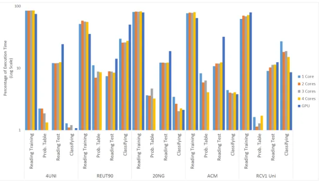
5.2 Efficiency of the steps of Naive Bayes algorithm implementation on CPU and GPU. . . 37

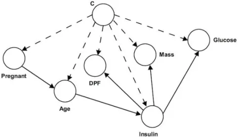
6.1 TAN model learned for the dataset “Pima”. . . 40

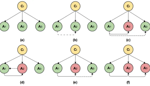
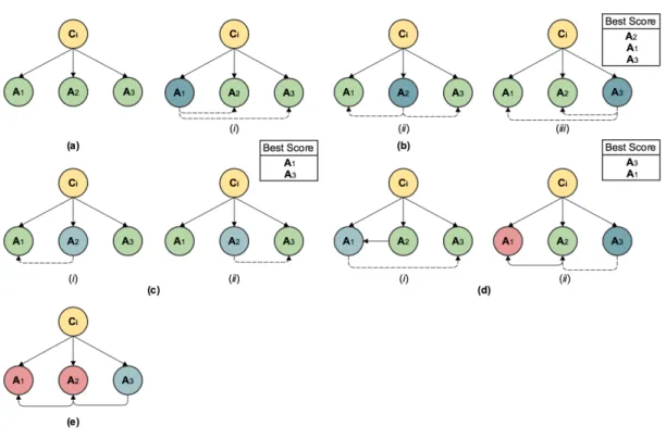
6.2 Example of the construction of the TAN. . . 41

6.3 Example of the construction of the SP-TAN. . . 42

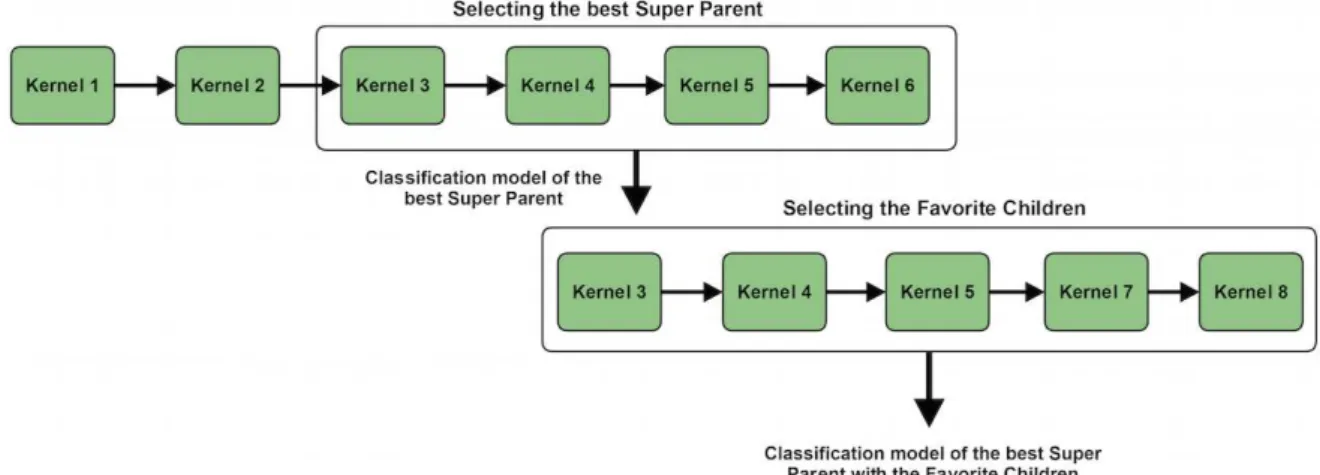
6.4 Execution of kernels . . . 47

(16)

(17)

List of Tables

2.1 Contingency Table for Classification Effectiveness Evaluation. . . 11

4.1 General information of the data collections. . . 29

4.2 Feature Weighting approaches applied on Naive Bayes Models. . . 31

4.3 Best results of Naive Bayes compared with SVM classifier. . . 32

6.1 Efficiency of the GPU-based implementation in select the best Super Parent - time in seconds. . . 50

6.2 Results of the LSPTAN strategies considering the Super Parent and Favorite Children. . . 51

6.3 Best results compared with SVM and KNN. . . 52

(18)

(19)

Chapter 1 Introduction

1.1 Context and Motivation

The amount of data created and shared nowadays in all types of platforms reached un-precedented levels, making the organization and extraction of useful knowledge from this huge amount of data one of the biggest challenges in Computer Science. Machine learning techniques, such as Automatic Document Classification (ADC), have demon-strated to be a viable path towards this goal. Particularly, ADC techniques aim at building effective models capable of associating documents with well-defined semantic categories in an automated way. ADC techniques are the core component of many important applications such as spam filtering (Hovold [2005]), organization of topic directories (Fahmi [2004]), identification of writing styles or authorship (Zheng et al. [2006]), among many others.

ADC methods usually exploit a supervised learning paradigm (Sebastiani [2002]), i.e., a classification model is first “learned” using previously labeled documents (training set), and then used to classify unseen documents (the test set). There is a plethora of supervised ADC algorithms available in the literature, such as Nearest-Neighbor clas-sifiers (Yang [1999]), Support Vector Machines (Fan et al. [2008]), boosting (Schapire and Singer [2000]) and Bayesian models (Manning et al. [2008]). In this work, we fo-cus on the latter approach, due to its simplicity, efficiency, and effectiveness in several scenarios. In particular, we focus on Naive Bayes approaches, the most widely used Bayesian paradigm for text classification.

Although being a widely used classification paradigm in ADC, other statistical learning methods, such as SVMs, have presented superior effectiveness than Naive Bayes approaches. The lack of robustness of NB is related to some characteristics present in real document collections, such as class imbalance and feature sparseness,

(22)

2 Chapter 1. Introduction

that may compromise some of the Naive Bayes premises (Rennie et al. [2003]; Kim et al. [2006]).

1.2 Master Thesis Hypotheses

In this section, we present the fundamental hypotheses used as guide for the construc-tion of the work:

• There is a combination of modeling and feature weighting that makes NB com-petitive with state-of-the-art classifiers in real scenarios.

• Alleviating or removing the premise of independence among attributes may im-prove the effectiveness of NB in real scenarios.

• Adopting new parallel techniques (e.g., GPU) may allow more efficient NB im-plementation.

• This parallel strategy may make feasible the execution of more complex Bayesian networks in real scenarios, since they are extremely expensive in large scenarios.

1.3 Work Description

Naive Bayes is often used as a baseline in text classification because it is fast and easy to implement. However, some characteristics present in text collections, such as class imbalance and feature sparseness may compromise the Naive Bayes classification effectiveness. First, class imbalance problem (Matthijssen [2000]) happens when the number of documents of one or few classes spams most of the documents in a dataset. This introduces a bias in the trained classifier towards assigning most unseen documents to the largest classes, incurring in a poor classification effectiveness in the minority classes, the most important ones in many applications (e.g. email spam, vandalism). Second, sparseness problem is related to the low frequency of certain features (i.e., terms/words) in some documents (Matthijssen [2000]). In Naive Bayes, the conditional probability of a termaj given a classci is estimated using all training documents from

ci in which aj occurs. Such conditional probabilities may be negatively affected if

aj occurs only in a few documents, especially in smaller classes (i.e., those with few

documents).

(23)

1.3. Work Description 3

and Oles [2000]; Rennie et al. [2003]; Adewole et al. [2014]) or by means of feature weighting strategies more adequate to ADC, in a preprocessing phase prior to the model construction (Kim et al. [2006]; Matthijssen [2000]). Although both research lines may produce significant improvements in the Naive Bayes effectiveness, when compared to its original version, the resulting methods are still not capable of surpass-ing some state-of-the-art ADC method such as SVMs. Thus, as ourfirst contribution

we present a broad and original (never reported) study on the combination of different Naive Bayes-based learning models with different feature weighting strategies, evaluat-ing these combinations in several real-world datasets. Our experimental results show that a proper combination of learning paradigms and weighting strategies may produce results comparable or even superior to SVMs in several datasets, at a lower cost.

A third research line that has been investigated in order to improve the Naive Bayes effectiveness are the so-called Semi-Naive Bayes methods, which relax the Naive Bayes attribute independence assumption (Manning et al. [2008]), by reduction of data (Chen and Wang [2012]) or, mainly, by means of extensions of the structure of the learning model to represent feature dependencies (Friedman et al. [1997]; Keogh and Pazzani [1999]). These strategies have produced gains when compared to NB in small datasets, such as those related to bioinformatics. However due to their high com-putational cost, inherent to the complexity of representing the term dependencies, they cannot scale to large classification tasks. Thus, investigating whether the relaxation of the Naive Bayes attribute independence assumption is effective in large ADC tasks is still an open problem. In this context, we present our second and third contribu-tions. The second contribution corresponds to an exclusive parallel version of the Naive Bayes approach using graphic processing units (GPUs). This parallel version allowed us to implement some Semi-Naive Bayes approaches, capable of running in large text collections. Thus, our third contribution is an original study about the impacts of the relaxation of the Naive Bayes assumption in large ADC tasks. In this investigation, we also introduce four original parallel lazy Semi-Naive Bayes strategy proposals which exploit the information of the document to be classified to reduce the complexity of the Semi-Naive Bayes learned model. Our experimental results point out that further improvements can be obtained with these models, depending on some dataset characteristics.

(24)

4 Chapter 1. Introduction

relax the Naive Bayes independence assumption in large ADC tasks? and (Q3) If yes for (Q2), are these Semi-Naive Bayes proposals capable of improving even further the best combinations found in the answer of (Q1)?

1.4 Contributions

The main contributions of the work are:

1. a thorough study on the aforementioned combinations of Naive Bayes Strategies and feature weighting approaches in five widely ADC datasets. More specifically,

• We review some proposals in the literature that try to overcome the ADC idiosyncrasies, either by proposing some changes in the construction of the Naive Bayes learning model (Rennie et al. [2003]; Zhang and Oles [2000]; Adewole et al. [2014]) or by means of feature weighting strategies more adequate to the ADC task, in a preprocessing phase prior to the construction of the model (Kim et al. [2006]; Matthijssen [2000]).

• We proposed a methodology that enables a deeper study of the impact of these Naive Bayes strategies (Rennie et al. [2003]; Zhang and Oles [2000]; Adewole et al. [2014]) when combined with the feature weighting approaches (Kim et al. [2006]; Matthijssen [2000]). We applied these combinations into five real textual collections and compared with two ADC algorithms.

2. the proposal and implementation of a parallel version of the Naive Bayes algo-rithm using graphic processing units (GPUs). This parallel version allowed us to build a more complex Bayesian network, capable of running in large collections.

3. the proposal of new GPU-based lazy Semi-Naive Bayes approaches. Again, more specifically,

• The introduced GPU-based parallel strategy of the Naive Bayes algorithm on the previous contribution allowed us to alleviate the independence assump-tion between the attributes, allowing us to build a more complex Bayesian network.

(25)

1.5. Roadmap 5

1.5 Roadmap

The remainder of this work is organized as follows.

Chapter 2 In this chapter, we briefly describe the supervised ADC task, some evalu-ation strategies and the GPU parallelism. We also present some of the notevalu-ation conventions adopted in this work.

Chapter 3 In this chapter, we describe related works. We start by describing some problems found in Text Classification. Then we discuss the strategies proposed in the literature that seek to alleviate these problems. We distinguish three broad areas for doing so: applying feature weighting, modifying the structure of the Naive Bayes and extending the Naive Bayes model by alleviating the independence between attributes. Finally, also discussed the use of parallelism through the graphics processing units in machine learning techniques.

Chapter 4 In this chapter, we describe the Naive Bayes learning paradigms and the several weighting schemes we exploit. We provide an extensive combination of proposed feature weighting strategies with different Naive Bayes models. We also describes our experiments over theses approaches applied in five real textual datasets.

Chapter 5 In this chapter, we describe our GPU-based parallel implementation of the Naive Bayes algorithm.

Chapter 6 In this chapter, we describe and evaluate our four Semi-Naive Bayes ap-proaches based on the several Semi-Naive Bayes we study. We start by introduc-ing the Semi-Naive Bayes which we based and the proposintroduc-ing strategies. We also describe our GPU-based parallel implementation of these Semi-Naive Bayes.

(26)

(27)

Chapter 2 Basic Concepts and Settings

In this chapter, we briefly describe what is automatic document classification and assessment strategies adopted throughout the work. We also present the parallelization environment (GPU - CUDA), which was adopted to implement the strategies presented in this master thesis.

2.1 Automated Document Classification

ADC methods usually exploit a supervised learning paradigm (Sebastiani [2002]), i.e., a classification model is first “learned” using previously labeled documents (training set), and then used to classify unseen documents (the test set). Let di = (~x, ci) be

a document, where ~x denotes its vectorial (bag of words) representation and ci is a

categorical attribute from a finite set ci ∈ C indicating its class (C is a finite set

composed by all the possible classes). In a probabilistic perspective, the main goal of ADC algorithm is to learn a discrete approximation of the class a posteriori probabil-ity distribution P(ci|di) that underlies the relationships between documents and their

associated classes. This probability distribution is learned according to a training set composed by already classified documents. There are two approaches for doing so, either based on a direct estimation of P(ci|di), or based on an indirect estimation of

P(ci|di).

The first approach is called discriminative classifier and it tries to model depen-dency on the observed data without making any assumption regarding the probability density function for each class. It makes fewer assumptions on the distributions. On the other hand, a generative classifier tries to learn the model by estimating the condi-tional probability and the prior probability to estimate the class posteriori probability distribution P(ci|di). In this case, one should assume a model for the class

(28)

8 Chapter 2. Basic Concepts and Settings

ties P(di|ci) and its parameters are estimated from the training set. For example, a

normal distribution may be chosen, and its mean and variance parameters are esti-mated according to the already classified data. Then the class a posteriori probability distributionP(ci|di)is estimated according to the Bayes’ rule:

P(ci|di) =

P(ci)·P(di|ci)

P

c′_∈_CP(c′)·P(di|c′)

whereP(c) is the prior probability and P(di|ci) is the conditional probability.

We assume c = f(~x) for some unknown function f, and the goal of learning is to estimate the function f given a labeled training set, and then to make predictions usingˆc= ˆf(~x). The quality of such approximation is based on how wellfˆpredicts the class of unseen documents. Clearly, a function fˆthat accurately predicts all training documentsD _{may not be accurate to predict the classes of unseen documents. In this}

case, we sayfˆis overfitted w.r.t. D_{. Hence, there exist a trade-off between complexity}

(the more complexfˆis, more specific patterns observed in the training set are learned) and generalization power offˆ(the more specific patterns observed in unseen documents may not be observed inD_).

It has been already proved that, asymptotically, discriminative classifiers are su-perior to generative ones (Vapnik [1998]), with several reported experiments corroborat-ing this findcorroborat-ing (Drummond [2006]). Indeed, if there are not enough traincorroborat-ing examples, the parametric model is deemed to overfit, decreasing its generalization power (Hastie et al. [2001]). However, some authors claim, based on experimental evaluation, that with realistic training set sizes, the generative classifiers may also perform as well as or better than discriminative ones. This comes true if the assumed parametric model used by the generative classifier is correct. In this case, the class priors become a useful information which is ignored by the discriminative classifiers. In this work we show that our generative classifier was able to outperform the discriminative classifiers (SVM and KNN).

2.1.1 ADC Classifier

We selected two representative and widely used ADC algorithms as baselines in our study. These algorithms are:

KNN: a lazy classifier that assigns to a test document d~test= (w1,j, w2,j, ..., wV,j), the

(29)

2.1. Automated Document Classification 9

As well as having a k value that is too small it is important to choose a value that isn’t too large as it can also lead to misclassification.

KNN determines the decision boundary locally, considering each training doc-ument independently. Here, we use cosine similarity to determine the nearest neighbors of a test document. The cosine similarity is measured by Equation 2.1.

cos(dneighborj, dtest) =

~

dneighborj •d~test

|dneighbor~ j| × |d~test|

(2.1)

The similarity of cosine of neighbors that belong to the same classciare grouped.

The class that express the highest similarity is the chosen one. Thus, the KNN’s decision function is expressed by the Equation 2.2.

cmap =argmax ci∈C

" _K X

j=1

cos(dneighborj, dtest)×λi #

(2.2)

where λi = 1 if dneighborj belong to ci. Otherwise, λi = 0.

Support Vector Machine (SVM): the SVM classifier aims at finding an optimal separating hyperplane between positive and negative training documents, max-imizing the distance (margin) to the closest points from both class. Given N training documents represented as pairs (xi, yi), where xi is the weighted feature

vector of the ith _{training document and} _y

i ∈ −1,+1 the set membership of the

document, SVM tries to maximize the margin between them on the training data, which leads to better classification effectiveness on test data. We may state the problem as

min

β,β0

1 2||β||

2 _{subject to} _y

i(xTi β+β0)≥1, (2.3)

where β is a vector normal to the hyperplane (the so-called weight vector),β0 is its intercept, and 0≤i≤N.

After introducing Lagrange multipliers αi (0 ≤ i ≤ N) for each inequality

con-straints in Equation 2.3, along with slack variablesξito account for non-separable

(30)

LP =

1 2||β||

2₊_C

N

X

i=1 ξi−

N

X

i=1

αi[yi(xTi β+β0)−(1−ξi)]− N

X

i=1

µiξi, (2.4)

which we minimize with respect toβ,β0 andξi, whereµiare Lagrange multipliers

employed to enforce ξi > 0. Setting the corresponding derivatives to zero, this

yields:

β =

N

X

i=1

αiyixi (2.5)

0 =

N

X

i=1

αiyi (2.6)

αi =C−µi, (2.7)

whereαi ≥0,µi ≥0andξi ≥0,∀i. By substitution into 2.4, we get the so-called

Lagrangian Wolfe (dual) function:

LD = N

X

i=1 αi −

1 2 N X i=1 N X j=1

αiαjyiyjxTi xj.

Furthermore, the solution must satisfy the Karush-Kuhn-Tucker (KKT) condi-tions, which include, along with Equations 2.5, 2.6 and 2.7, the following ones:

αi[yi(xTi β+β0)−(1−ξi)] = 0

µiξi = 0

yi(xTi β+β0)−(1−ξi)≥0,

(2.8)

where 0≤i≤N.

Finally, the solution for β is βˆ = PN

i=1αˆiyixi, with non-zero αˆi for support

points which lie in the support vectors. The solution for β0 may be devised by Equation 2.8, normally averaging the solutions regarding the support points to achieve numerical stability.

Thus, we can express the SVM’s decision function as:

ˆ

(31)

2.2. Evaluation Techniques 11

where the sign of the score is used to predict the example’s class. Since SVM is a binary classifier, it should be adapted to handle multiclass classification problems. The two most common strategies for doing so are the one-against-one and the one-against-all (Manning et al. [2008]).

2.2 Evaluation Techniques

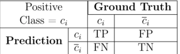
An important aspect to be considered is how to evaluate the effectiveness of a classifier (that is, its accuracy in classifying unseen data or, in other words, its generalization power), assessed by first learning a classification model based on the training set and then applying it to classify a set of unseen documents (the test set). Some measures of classification effectiveness are then used to assess the quality of the classification model learned. Several measures for this purpose were proposed in the literature and some of them are widely used by the Machine Learning community. Among the most used measures are precision, recall and F1 measure. In order to describe each of these measures in a binary classification, let’s consider the contingency table represented in Table 2.1 (also known as confusion matrix), where TP, TN, FP and FN denote, respec-tively, the number of true positives, true negatives, false positives and false negatives, defined as:

True Positive (TP): positive test document correctly classified into the positive class.

True Negative (TN): negative test document correctly classified into the negative class.

False Positive (FP): negative test document incorrectly classified into the positive class.

False Negative (FN): positive test document incorrectly classified into the negative class.

The precisionpof a performed classification denotes the fraction of all documents assigned to the positive class ci by the classifier that really belong to ci. In terms of

the contingency table, this translates into

p= T P

(32)

Positive Ground Truth

Class =ci ci ci

Prediction ci TP FP

ci FN TN

Table 2.1: Contingency Table for Classification Effectiveness Evaluation.

The recall r of a performed classification denotes the fraction of all documents that belong to the positive class ci that were correctly assigned to ci by the classifier.

Again, in terms of the contingency table, this can be expressed as

r = T P

T P +F N

Finally, the F1 measure is defined as the harmonic mean of the precision and the recall, given by

F1 = 2pr

p+r

There are two conventional methods to evaluate classification algorithms when applied to problems with more than two classes, namely by micro-averaging and macro-averaging theF1measure. The micro-averagedF1 (MicroF1) is calculated from a global contingency table (similarly to Table 2.1), with the precision and recall being calculated as a sum of each entry of the table:

pmicro =

P|C|

i=1T Pi

P|C|

i=1T Pi+F Pi

rmicro =

P|C|

i=1T Pi

P|C|

i=1T Pi+F Ni

In contrast, the macro-averaged F1 (MacroF1) is calculated by first calculating the precision and recall values for each class and computing their average value:

pmacro =

1

|C|

X

i=1

T Pi

T Pi+F Pi

rmacro=

1

|C|

X

i=1

T Pi

T Pi+F Ni

(33)

2.3. GPU and CUDA 13

MacroF1 measure is a class pivoted measure that gives equal weights to the classes. Since the ADC task may be seen as a stochastic process, it is fundamental to adopt some evaluation strategies that guarantee the statistical validity of the obtained classification results, which is achieved by replicating the experiments using different training sets to learn a classification model. For this purpose, the cross validation strategy has become a standard in the machine learning community. There are, at least, two usual strategies for cross validation, the K-fold cross validation and the repeated random sub-sampling (Kohavi [1995]).

The K-fold cross validation consists of randomly splitting the data into K inde-pendent folds. At each iteration, one fold is retained as the test set, and the remaining K - 1 folds are used as training set. The repeated random sup-sampling consists of randomly selecting a fraction of documents from the dataset, without replacement, to compose the test set, and the remaining documents retained as the training set. This is performed for each replication. Since in the K-fold cross validation the size of the folds are dependent of the number of iterations, it becomes more suitable to medium/large sized datasets, while the repeated random sub-sampling is usually adopted to small sized datasets when the number of replications is large.

For more details on ADC and evaluation strategies, we refer the reader to Baeza-Yates and Ribeiro-Neto [2011]; Hastie et al. [2001]; Manning et al. [2008].

2.3 GPU and CUDA

General purpose parallel programming on GPUs is a relatively recent phenomenon. GPUs were originally hardware blocks optimized for a small set of graphics operations. As demand arose for more flexibility, GPUs became increasingly more programmable. Early approaches for computing on GPUs cast computations into a graphics framework, allocating buffers (arrays) and writing shaders (kernel functions). Several research projects looked at designing languages to simplify this task. In late 2006, NVIDIA introduced its CUDA architecture and tools to make data parallel computing on a GPU more straightforward. Not surprisingly, the data parallel features of CUDA map pretty well to the data parallelism available on NVIDIA GPUs.

(34)

for direct access to host memory from the GPU under certain restrictions. As a GPU is designed for stream or throughput computing, it does not depend on a deep cache memory hierarchy for memory performance. The device memory supports very high data bandwidth using a wide data path.

In 2007, NVIDIA saw an opportunity to bring GPUs into the mainstream by adding an easy-to-use programming interface, which it dubbed CUDA, or Compute Unified Device Architecture. This opened up the possibility to program GPUs with-out having to learn complex shader languages, or to think only in terms of graphics primitives (Cook [2013]).

CUDA is an extension to the C language that allows GPU code to be written in regular C. The code is either targeted for the host processor (the CPU) or targeted at the device processor (the GPU). The host processor spawns multithread tasks (or kernels as they are known in CUDA) onto the GPU device. The GPU has its own internal scheduler that will then allocate the kernels to whatever GPU hardware is present. We’ll cover scheduling in detail later. Provided there is enough parallelism in the task, as the number of SMs in the GPU grows, so should the speed of the program. CUDA, unlike its predecessors, has now actually started to gain momentum and for the first time it looks like there will be a programming language that will emerge as the one of choice for GPU programming. Given that the number of CUDA-enabled GPUs now number in the millions, there is a huge market out there waiting for CUDA-enabled applications.

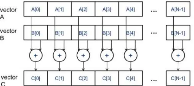
In CUDA, a kernel function specifies the code to be executed by all threads during a parallel phase. Since all these threads execute the same code, CUDA programming is an instance of the well-known SPMD - Single Program, Multiple Data (Atallah and Blanton [2010]) parallel programming style, a popular programming style for massively parallel computing systems. Figure 2.11

illustrates the concept of data parallelism with a vector addition example. In this example, each element of the sum vector C is generated by adding an element of input vector A to an element of input vector B. For example, C[0] is generated by adding A[0] to B[0], and C[3] is generated by adding A[3] to B[3]. All additions can be perform in parallel.

When a host code calls or launches a kernel, it is executed a large number of threads on a device. All threads that are generated by a kernel launch are collectively called a grid. Each grid is organized into an array of thread blocks. All blocks of a grid are of the same size and can contain up to 1,024 threads. The number of threads in each thread block is specified by the host code when a kernel is launched. Unique coordinates

1

(35)

2.3. GPU and CUDA 15

Figure 2.1: Data Parallelism in vector addition.

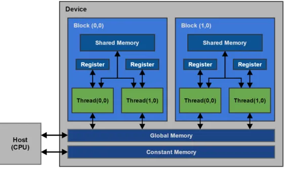
(blockIdx and threadIdx) variables allow threads of a grid to identify themselves and their domains of data. This model of programming compels the programmer to organize threads and their data into hierarchical and multidimensional organizations.

(36)

(37)

Chapter 3 Related Work

In this chapter we present the strategies proposed in the literature to deal with the problems discussed in the previous section. First, we present the strategies that per-form some adjustments in the Naive Bayes model, making it more robust for text classification. Then, we present the feature weighting approaches that are used to weight the attributes values of each document in the training set. Then, we present some proposals in the literature that extend the Bayesian model, alleviating the as-sumption of independence between attributes assumed by the Naive Bayes algorithm. These strategies are called Semi-Naive Bayes. Finally, we discuss the use of GPU-based parallel implementations in classification algorithms. These implementations are able to achieve high levels of parallelism and lower power consumption. A strategy that could be exploited in the Semi-Naive Bayes strategies, since they are extremely costly and unfeasible in terms of time execution when applied to real scenarios, such as real textual collections.

3.1 Naive Bayes Limitations

A fundamental assumption assumed by most automatic classifiers is that the data used to learn the classification model are random samples independently and identically distributed (i.i.d.) of a statistical distribution that governs the data. However, this may not be the case. Indeed, in many real scenarios the training data do not follow the same distribution of the test data, compromising the effectiveness of the classification algorithms.

The Naive Bayes algorithm is one of the most widely used techniques, due to its simplicity and efficiency in several scenarios, especially when applied to scenarios in which the attributes are independent, making their “ naive ” assumption more

(38)

18 Chapter 3. Related Work

liable. Normally in text classification, its effectiveness is not as good as some other statistical learning methods. This fact is related to some characteristics presented in real document collections, such as unbalanced data, sparsity, among others, that may compromise some of Naive Bayes premises.

In Rennie et al. [2003] and Kim et al. [2006], the authors described some prob-lems faced by the Naive Bayes classifiers, when applied to real textual scenarios. The principal factors are:

• Class imbalance • Document length • Feature sparseness

The unbalanced class problem (Witten and Frank [1999]) refers to scenarios where the number of documents of one or few classes far exceeds the number of documents in the other classes. The amount of documents in classes is an important factor, since it is related to the amount of information used to learn the classification model (P(di|ci)).

So, if the class has sufficient samples, the classifier can learn properly to classify new instances of that class. As for the minor classes, the lack of information inhibits the prediction of new samples, so that the classifier tends to classify them as samples of the majority class.

The document length is another important factor, which may affect in the ef-fectiveness of the classification, especially when this factor is combined with the class imbalance. Short documents are brief and the frequency of words is generally low, thus the relevant words occur once or twice in the document. In longer documents, words are more frequent, so relevant words usually occur more often in the document. Thus, when a collection has long and short documents, the relevant words of the short documents are negligible when compared with the relevant words of longer documents, since these are more frequent. Imagine the case where minority classes have a majority of short documents. In this case, the class has a much lower amount of information due to infrequency of documents and attributes. Thus, the estimateP(di|ci)for a test

document for the minority class will be hidden by the estimate of the majority classes, converging the classification of minority class documents to the majority classes.

3.2 Naive Bayes Strategies and Feature Weighting

(39)

classifica-3.2. Naive Bayes Strategies and Feature Weighting 19

tion scenarios. However, this simplicity in the construction of the classification models may significantly compromise the effectiveness of NB in some scenarios, such as tex-tual document classification. In Rennie et al. [2003], several disadvantages of the more traditional Naive Bayes Multinomial model (Manning et al. [2008]) are presented in real-world text collections. The authors argue that some characteristics of document collections such as imbalance among classes and data sparsity, significantly compro-mise the learning model proposed by the Naive Bayes method. Based on this study, the authors proposed a simple heuristic based on data transformations and simple ad-justments in the construction of the learning model, which was called Transformed Weight-normalized Complement Naive Bayes (TWCNB). The main idea of this heuris-tic is to perform a number of feature frequency transformations and adjustments in computing probabilities to improve the Naive Bayes modeling text classification. Fol-lowing this idea, Zhang and Oles [2000] presented another proposal for construction of models that combine Multinomial Naive Bayes with the technique one-versus-all (Zhang and Oles [2000]), widely used in multiclass classification scenarios. Basically this proposal uses the one-versus-all technique to balance information among classes, smoothing the imbalance.

A more recent study shows that smoothing Naive Bayes may improve the classi-fication performance (Adewole et al. [2014]), since smoothing aims to adjust the prob-ability of an unseen event, which arises due the data sparseness. According to Zhai and Lafferty [2001] smoothing may improve the reliability of Bayesian model, by as-signing non-zero probabilities to terms that do not occur in the document. Following this research strategy, the authors of Adewole et al. [2014] applied the concept of linear interpolation smoothing (Jelinek-Mercer smoothing) to Naive Bayes Spam Classifica-tion. This combination performed well at improving spam classification, also reducing false positives.

(40)

3.3 Semi-Naive Bayes

As mentioned earlier, Naive Bayes is based on the premise that feature occurrences in documents of different classes are independent (Manning et al. [2008]). The main reason for the adoption of this premise is the time complexity, since the construction of a complete and optimal Bayesian network is an NP-hard problem (Cooper [1988]). Thus, a strategy that has being considered (called semi-Naive Bayes) is based on heuris-tics that relax the assumption of independence without ensuring the optimal model. A number of semi-Naive Bayes methods have been proposed in recent years (Fried-man et al. [1997]; Keogh and Pazzani [1999]; Zhang et al. [2005]). They fall into two categories: data-based and structure-based methods. Those on the first category aim at choosing the training data such that the dependencies within the chosen data are weaker than those in the whole dataset. The local learning methods, such as Lazy Bayesian Rules (Zheng and Webb [2008]), accommodate violations of the independence assumption by choosing a desired set of the training samples on which Naive Bayes is applied. Another group of methods in the data-based category apply Naive Bayes on a subset of attributes. This is achieved by feature selection (Zheng et al. [2004]) which removes irrelevant and redundant attributes.

(41)

3.4. GPU parallelization 21

been evaluated yet.

3.4 GPU parallelization

A practical challenge common to all machine learning approaches is how to apply them in real scenarios, where the volume of data is typically huge and the characteristics of the collections vary significantly. Some of the most commonly used techniques to deal with such issues are dimensionality reduction by feature selection (Zheng et al. [2004]), whose goal is to keep only the features that better “define” the documents, and data indexing (Christen [2012]; Cha and Yoon [2002]), whose goal is to represent the data in a more direct and efficient way. Another solution that has been adopted to address these issues is to exploit parallel computation, either by means of distributed mem-ory strategies (Ruocco and Frieder [1997]; Kruengkrai and Jaruskulchai [2002]), or by means of massive parallelism through graphic processors (Kumarihamy and Arundhati [2009]; Grahn et al. [2011]; Lin and Chien [2010]; Garcia et al. [2008]; Andrade et al. [2013]). This last group of strategies has recently demonstrated very interesting results, since they are capable of producing parallelism levels much higher than those achieved by CPUs, associated with a smaller energy consumption (Timm et al. [2010]).

(42)

3.5 Chapter Summary

(43)

Chapter 4 Combining Learning Models and

Feature Weighting Strategies

4.1 Naive Bayes Learning Models

As previously mentioned, some premises of the traditional NB model are significantly compromised by some characteristics of real text collections, such as the class imbalance and the term sparseness. In this Section, besides presenting the traditional Naive Bayes, we introduce some of the most important extensions aimed at making it more resilient to the problems presented in Chapter 3. All the models presented in this Section are used in our experimentation.

4.1.1 “Traditional” Naive Bayes

The Naive Bayes (Manning et al. [2008]) calculates the “score” of a class ci as the

prob-ability of a documentdt being assigned to classci. Based on this score, a class ranking

is created and NB assigns to dt the class in the top of the ranking. More formally, let

P(ci|dt)be the probability of a test documentdt(a1, a2, . . . , aj)to belong to theciclass,

where (a1, a2, . . . , aj)is a feature vector (binary or weighted) representing the term set

of document dt. This probability is calculated using the Bayes Theorem. However,

the calculation of P(ci|dt) has a high computational cost, given that the number of

possible vectors dt is very high due to the potential number of term dependencies. To

attenuate this problem, the NB algorithm assumes that the occurrence of all terms is independent from each other (the NB independence assumption), a simplification that makes the classification problem computationally viable. Thus, P(ci|dt)is defined as:

(44)

24

Chapter 4. Combining Learning Models and Feature Weighting Strategies

P(ci|dt) =

P(ci)Q_∀_j_∈_d_tP(aj|ci)

P(dt)

(4.1)

By observing Equation 4.1, we see that the fundamental question in the P(ci|dt)

definition is how to estimate P(aj|ci). Thus, according to Manning et al. [2008], we

define:

P(aj|ci) =

T ci(aj) +α

P

v∈V T ci(v) +α· |V|

where T ci(aj) is the number of occurrences of term aj in class ci and P_v_∈VT ci(v) is

the summation of the occurrences of all terms in documents belonging toci. To avoid

inconsistencies (e.g., division by zero), a weighted Laplace smoothing is usually applied, consisting of an addition of an α parameter to the numerator and as a multiplication factor to the vocabulary size in the denominator.

In ADC, the goal is to find the “best” class for dt, usually defined as the one

with the highest conditional probability. To avoid computational precision losses (e.g., due to floating point underflow), it is usually more adequate to add the log of the probabilities instead of performing the previously defined multiplication. Thus, this maximization, in most NB implementations is defined as:

cmap =argmax ci∈C



logP(ci) +

X

1≤j≤|V|

logP(aj|ci)



 (4.2)

4.1.2 Interpolated Naive Bayes

(45)

4.1. Naive Bayes Learning Models 25

(P(aj|ci)) along with the estimates of aj in the collection (P(aj)). Thus, the authors

substitute the original formula 4.2 by the formula 4.3.

cmap =argmax ci∈C

"

logP(ci) +

X

1≤j≤|V_|

λ·logP(aj) + (1−λ)·logP(aj|ci)

#

(4.3)

4.1.3 One versus All Naive Bayes

In Zhang and Oles [2000], the authors proposed another solution to the class imbalance problem. This strategy consists of combining the One versus All (OVA) strategy, commonly used in binary classifiers such as SVMs for solving multiclass classification problems, to the traditional NB classifier. The OVA strategy reduces a multiclass problem to a binary one, by considering one class as the positive and the union all others as the negative one. Thus, the OVA-NB uses more information to build the classification model for each class, favoring minority classes.

To accomplish the OVA strategy into NB, the complement of the probability for a given class P(aj|ci), is used. More formally, to calculate the complement of the

probability of a term aj in a given class ci, we use the information contained in all

classes but ci, as follows:

P(aj|ci) =

T ci(aj) +α

P

v∈V T ci(v) +α·V

where, T ci(aj) is the number of occurrences of term aj in all classes but ci and

P

v∈VT ci(v) is the summation of the number of occurrences of all terms in the

doc-uments of all classes, but ci. To avoid inconsistencies in the probability estimates, a

Laplace weighting strategy is also adopted. Due to imbalance issues, which may be exacerbated by the union of the “negative” classes, the apriori estimate of the class is not used in this model. The OVA-NB classification model is summarized as:

cmap =argmax ci∈C



 X

1≤j≤|V|

logP(aj|ci)−logP(aj|ci)



(46)

26

4.1.4 Complement Naive Bayes

Finally, in Rennie et al. [2003], the authors proposed the Complement Naive Bayes (CNB) learning model, exploited in the TWCNB proposal. Actually, CNB is an exten-sion of OVA-NB in which, instead of calculating the P(dt|ci) using information from

ci, the CNB uses only the complement of the probability P(dt|ci). This complement

balances the information used in the learning model, not favoring the majority classes.

cmap =argmax ci∈C



 X

1≤j≤|V_|

−logP(aj|c¯i)





4.2 Feature Weighting Strategies

In this section, we present some of the main feature weighting strategies used by Bayesian models in order to overcome problems related to the imbalance and spar-sity of real textual collections.

4.2.1 Term Frequency

One of the main assumptions made in ADC is that, by means occurrence frequen-cies of terms, it is possible to determine the topic of a text. A term that occurs more frequently in a given document is more important than an infrequent term. The term frequency (tf) measures the number of occurrences of a term in each single text document (Matthijssen [2000]). Although it is the simplest weighting strategy, tf is commonly used in ADC.

(47)

4.2. Feature Weighting Strategies 27

4.2.2 Product of the term and inverse document frequency

(tf-idf)

After elimination of stopwords, a document still may contain many terms that are poor indication of a class. Common terms tend to occur in numerous documents in a collection and are often randomly distributed over all of them. The importance of a term is related to the number of documents in which it occurred. The more documents a term occurs, the less important it may be. For instance, the term “computer” is not a discriminative term in a document collection computing, no matter what its overall frequency.

Therefore, a commonly adopted premise is that the more rarely a term occurs in a collection, the more discriminative a term is. Thus, the weight of the term should be inversely related to the number of documents in which the term occurs. An inverse document frequency (idf) factor is commonly used to represent this effect. In this case, the logarithm smooth the effect of the inverse document frequency factor.

log

N ni

On the other hand, the frequency of the term within the document (tf) should be considered as measure of importance of the term in the collection. This suggests that the relevance of a term in a document can be measured by the product of frequency of occurrence (tf or log(tf)) of the term within the document by the inverse document frequency factor of the term. This feature weighting method is known as tf −idf:

tfi·log

N ni

4.2.3 Relative Frequency

Relative Frequency is a length normalization method that normalizes the term fre-quency by dividing it by a normalization factor given by the maximum frefre-quency of a term occurring in any text document of the collection, as shown in Equation 4.4.

RF = tfi

N F (4.4)

(48)

28

collection, i.e.,N Fu =α·avdu+ (1−α)·duj, whereavduindicates the average number

of unique terms in a document over the collection andduj means the number of tokens

and unique terms in a documentdj. This linear interpolation smoothies the length of

each document using the characteristics of document collection.

RFu =

tfi

N Fu

(4.5)

The Relative Frequency method based on unique terms (Equation 4.5) signifi-cantly has increased the effectiveness of Naive Bayes algorithm (Kim et al. [2006]), proving to be more effective than BM25 (Robertson et al. [1999]) and PLN (Singhal et al. [1999]) methods.

4.3 Experimental Evaluation

4.3.1 Datasets

In order to evaluate the selected combinations, we consider five real-world textual datasets, namely, 20 Newsgroups; Four Universities; Reuters; ACM Digital Library and RCV1 datasets. We performed a traditional preprocessing task for all datasets: we removed stopwords, using the standard SMART list, and applied a simple feature selection by removing terms with low “document frequency (DF)”1

. Next, we give a brief description of each dataset.

4 Universities (4UNI), a.k.a, WebKB this dataset contains Web pages col-lected from Computer Science departments of four universities by the Carnegie Mellon University (CMU) text learning group. There is a total of 8,277 web pages, classified into 7 categories (such as student, faculty, course and project web pages).

Reuters (REUT90) this is a classical text dataset, composed by news articles collected and annotated by Carnegie Group, Inc. and Reuters, Ltd. We consider here a set of 13,327 articles, classified into 90 categories.

ACM-DL (ACM)a subset of the ACM Digital Library with 24,897 documents

containing articles related to Computer Science. We considered only the first level of the taxonomy adopted by ACM, where each document is assigned to one of 11 classes.

20 Newsgroups (20NG)this dataset containing 18,805 newsgroup documents, partitioned almost evenly across 20 different newsgroups categories. 20NG has become a popular dataset for experiments in text applications of machine learning techniques, such as text classification and text clustering.

1

(49)

4.3. Experimental Evaluation 29

RCV1 Uni The Reuters Corpus Volume 1 (RCV1) is a dataset with 804,427

English language news stories. We considered the complete topics taxonomy comprised of 103 classes. However, the original RCV1 is a multilabel dataset with the multilabel cases needing special treatment, such as score threshold, etc. (see Lewis et al. [2004] for details). As our current focus is on unilabel tasks, to allow a fair comparison among the other datasets (which are also unilabel) and all baselines (which also focus on unilabel tasks), we decided to transform all multilabel cases into unilabel ones. In order to do this fairly, we randomly selecting, for each documents with more than one label, a single label to be attached to that document. This procedure was applied in about 20% of the documents of RCV1 which happened to be multilabel.

Collections Distribution of the Classes Number of Number of

Classes Minor Class Median Mean Major Class Attributes Documents

4UNI 7 137 930 1.182 3.759 40.195 8.277

REUT90 90 2 29 148,1 3.964 19.590 13.327

20NG 20 628 979 940,2 999 61.050 18.805

ACM 11 63 2.041 2.263,36 6.562 56.449 24.897

RCV1 Uni 103 91.399 165.850 201.107 381.328 155.796 804.427

Table 4.1: General information of the data collections.

4.3.2 Evaluation, Algorithms and Procedures

The Naive Bayes models were compared using micro averaged F1 (MicF1) and macro averaged F1 (MacF1), standard information retrieval measures (Lewis et al. [1996]; Yang [1999]; Yang and Pedersen [1997]). While the MicF1 measures the classification effectiveness over all decisions (i.e., the pooled contingency tables of all classes), the MacF1 measures the classification effectiveness for each individual class and averages them. All experiments were executed using a 5−fold cross-validation (Breiman and Spector [1992]) procedure. The parameters were set via cross-validation on the training set2

, and the effectiveness of the algorithms, running with distinct types of features, were measured in the test partition. To compare the average results on our cross-validation experiments, we assess the statistical significance of our results by means of a paired t-test with 95% confidence. This test assures that the best results, marked in bold, are statistically superior to others..

2

(50)

30

In order to evaluate the performance of different Naive Bayes model combined with different feature weighting approaches, we compare then with SVM and KNN classifiers. Regarding SVM classifier, we adopt the LIBLINEAR (Fan et al. [2008]) implementation, using a linear kernel on which the regularization parameter was chosen among eleven values from2−5 _to ₂15 _{by using} ₅_{−fold cross-validation on each training} dataset. In the KNN classifier, the size of neighborhood was set via cross-validation in the training set. We also tested the four described feature weighting schemes with KNN, SVM. The best overall results for SVM and KNN were obtained using thelog(T F)− IDF weighting scheme, therefore these versions will be used as baselines.

All experiments were run on a Quad-Core Intel Xeon E5620, running at 2.4GHz, with 16Gb RAM. The GPU experiments were run on a GeForce GTX TITAN Black, with 6Gb RAM. The machine was reserved to execute each of the experiments indi-vidually, to guarantee accuracy of the efficiency results for each implementation.

We would like to point out that some of the results may differ from the ones reported in other works for the same datasets (e.g., Kim et al. [2006]; Rennie et al. [2003]; Godbole and Sarawagi [2004]). Such discrepancies may be due to several factors such as differences in dataset preparation3

; the use of different splits of the datasets (e.g., some datasets have “default splits” such as REUT90 and RCV14

), the application of some score threshold, such as SCUT, PCUT, etc., which, besides being an impor-tant step for multilabel problems, also affects classification performance by minimizing class imbalance effects, among other factors. We would like to stress that we ran all alternatives under the same conditions in all datasets, using standardized and well ac-cepted cross-validation procedures that optimize parameters for each alternatives, and applying the proper statistical tools for the analysis of the results. All our datasets are available for others to replicate our results and test different configurations.

4.3.3 Results

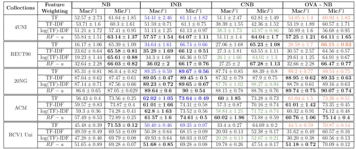
Table 4.2 shows the results of all selected combinations. For each dataset, we tested the four described feature weighting strategies along with the four discussed NB variants. The colors indicate the results for the methods as originally proposed: bluecorresponds to INB which used the TF weighting scheme, green corresponds to the original pro-posal of the CBN using log(TF)-IDF and finally,red corresponding to OVA-NB which originally exploited the TF scheme.

3

For instance, some works do exploit complex feature weighting schemes or feature selection mech-anisms that do favour some algorithms in detriment to others.

4

(51)

4.4. Chapter Summary 31

Overall, we can observe in the Table that the combination of the IN B learning model with the RF −u weighting strategy produced the best results in all datasets. We can also observe that the use of the RF −u strategy produced some expressive gains over the other weighting strategies in several cases (e.g., MacF1 forOV A−N B in RCV1 and MacF1 for NB in Reuters). It can also be observed that the use of this same weighting strategy resulted in some gains in the best learning model INB), such as the statistically significant gains in MacF1and MicF1in4U N I over the other strategies.

Table 4.3 presents a comparison among SVM, KNN and the best NB approach for each collection. We can see that most of the results of Best-NB (4 out of 5) uses the weighting strategyRF−u, three with the INB and one of the OVA-NB learning models. Only for the ACM dataset the best results were achieved withlog(T F)−IDF+IN B. But even in these cases, the combination RF −u+IN B was very close to the best results. In fact, there is a statistical tie in ACM. Notice that the best combination for a particular dataset can be determined in the validation set. This is very feasible, especially due to the NB efficiency.

We can see in Table 4.3 that the Best-NB combination outperforms or ties with KNN in eight out of ten cases (six wins and two ties). When compared to SVM, the Best-NB ties or outperforms this classifier also in eight out of ten cases (seven wins and one tie), loosing in other two (regarding MicF1). In fact, if we look at the MacF1results, Best-NB outperformed or tied SVM and KNN in all five datasets. This is consistent with the fact that most of the learning models and weighting scheme adaptations were designed to deal with the class imbalance issue, which tends to favor MacF1.

Thus, we conclude that, if good performance across all classes, mainly the mi-nority ones, is the main goal for a particular application, our results demonstrate that there is probably a combination of a NB learning model and a weighting strategy (most probably RF −u+IN B) that may deliver a top-notch performance.

4.4 Chapter Summary

(52)

32

Collections _WeightingFeature _Mac_F1 NB _Mic INB CNB OVA - NB

F1 MacF1 MicF1 MacF1 MicF1 MacF1 MicF1

4UNI

TF 52.57±2.73 61.64±1.85 54.41±2.46 61.11±1.82 51.1±2.47 62.81±1.49 54.85±1.4 60.93±1.83 TF-IDF 53.71±1.6 60.3±1.61 51.59±0.71 61.1±0.75 38.39±1.55 42.36±1.52 53.19±1.89 60.57±1.71 log(TF)-IDF 51.21±1.72 57.41±0.95 51.13±1.25 61.13±0.97 38.3±1.73 43.87±0.86 50.89±1.6 56.68±0.95 RF−u 55.84±1.51 63.14_±1.37 57.57_±1.54 64.07_±1.11 _51.11_±_1.4 64.04_±1.7 57.25_±1.21 64.11_±1.65

REUT90

TF 16.17±1.06 65.39±1.09 34.64±1.61 66.74±0.66 27.06±1.68 65.23±1.08 28.58±1.7 66.15±0.63 TF-IDF 23.62±0.64 65.58±0.81 35.29±1.69 66.12±0.51 27.3±1.81 63.55±1.11 30.57±2.57 64.56±0.57 log(TF)-IDF 19.23±1.44 65.61±0.88 34.3±1.68 66.36±0.57 26.1±1.66 64.01±1.3 29.61±1.25 64.91±0.67 RF−u 32.64±2.28 66.03±0.82 36.02±2 66.17±0.76 27.25±2 67.28±1.13 32.66±2.28 66.47±0.77

20NG

TF 85.31±0.81 86.0.4±0.82 89.25±0.59 89.67_±0.56 _87.74_±_0.85 _88.39_±_0.8 _89.2_±_0.77 _89.54_±_0.75

TF-IDF 87.04±0.62 87.47±0.61 89.05_±0.47 89.45_±0.5 _87.32_±_0.79 _87.9_±_0.75 88.95_±0.62 89.33_±0.63 log(TF)-IDF 87.14±0.71 87.56±0.66 89.23_±0.72 89.65_±0.67 ₈₇.76±1.02 88.27±0.94 88.78±0.61 89.16±0.63

RF−u 86.6±0.65 87.05±0.629 89.64_±0.6 90_±0.54 _88.15_±_0.78 _88.76_±_0.76 89.74_±0.75 90.07_±0.74

ACM

TF 56.43±0.4 73.56±0.25 62.02±1.05 73.64±0.49 60±1.85 73.28±0.73 61.04±1.5 73.26±0.51 TF-IDF 59.57±0.83 73.87±0.4 61.01±1.66 74.31±0.58 57.3±0.87 70.16±0.74 61.01±1.42 73.35±0.45 log(TF)-IDF 59.3±0.36 74.28±0.41 62.8±1.63 73.52±0.56 58.84±1.25 71.72±0.74 60.32±0.91 74.12±0.48 RF−u 57.49±0.53 72.89±0.25 61.57±1.6 74.61±0.5 60.02±1.96 73.88±0.59 60.76±1.06 75.14±0.4

RCV1 Uni

TF 45.48±0.39 71.53_±0.12 ₅₀.40±0.46 69.35±0.07 33.4±0.27 64.69±0.2 44.5±0.59 70.87±0.14 TF-IDF 49.59±0.49 69.53±0.09 50.38±0.64 68.15±0.09 20.93±0.13 52.38±0.17 31.62±0.49 60.57±0.16 log(TF)-IDF 47.28±0.46 69.79±0.08 49.93±0.64 68.03±0.07 20.28±0.13 52.07±0.21 30.20±0.38 60.56±0.13 RF−u 51.65±0.89 69.28±0.07 51.68_±0.85 _69.28_±_0.08 _19.78_±_0.26 _47.51_±_0.17 51.18_±0.72 _70.09_±_0.12

Table 4.2: Feature Weighting approaches applied on Naive Bayes Models.

Collections SVM KNN Best-NB Best-NB (Source)

MacF1 MicF1 MacF1 MicF1 MacF1 MicF1

4UNI 56_.02_±2_.02 ₇₀_.₉₁_±₁_.₉ 58_.24_±2_.92 73_.78_±0_.7 57_.57_±1_.54 ₆₄_.₀₇_±₁_.₁₁ _RF₋_u₊_{IN B} REUT90 30.38±2.04 65.09±0.21 29.95±1.14 68.04_±0.62 36.02_±2 66.17_±0.76 RF−u+IN B

20NG 84.92±0.54 85.1±0.6 88.41±0.27 88.69±0.67 89_.74_±0_.75 90_.07_±0_.74 _RF₋_u₊_{OV A}₋_{N B} ACM 58.00±1.33 69.67±0.45 59.75±1.72 71.6±0.46 62.8_±1.63 73.52_±0.56 log(T F)−IDF+IN B RCV1 Uni 47.05±0.35 75_.85_±0_.08 ₄₆_.₃₂_±₀_.₇₂ ₆₈_.₂₃_±₀_.₁₆ 51_.68_±0_.85 ₆₉_.₂₈_±₀_.₀₈ _RF₋_u₊_{IN B}

Table 4.3: Best results of Naive Bayes compared with SVM classifier.

(53)

Chapter 5 Parallelization of Naive Bayes

Classifier Using GPU

Over the last years, the computer industry has shifted from pushing clock frequency to parallelism. Rather than increasing the speed of its individual processor cores, traditional CPUs have increased the number of cores (multicore processors) as the primary basis for increasing system performance. This trend has also been followed by many core GPU chips which have now thousands of processing cores. The general perception is that processors are not getting faster, but instead are getting wider, and the only way to improve performance is through the exploitation of parallelism.

CPUs are optimized for low-latency access and excel in running single-threaded processes whereas GPUs are optimized for high throughput and can deal with mas-sive multithreaded parallelism. GPUs can handle masmas-sive amounts of data, which is critical for Information Retrieval (IR), however its different architecture and memory hierarchy requires the design of novel algorithms and new implementation approaches. This situation has hampered the exploitation of this opportunity by the IR commu-nity. However, recent works on Database Scalability, Document Clustering, Learning to Rank, Big Data Analytics and Interactive Visualization (Chang et al. [2012]; Teitler et al. [2014]; Shchekalev [2014]; Netzer [2014]; Graham and Mostak [2014]) have pro-duced some encouraging results.

The probabilistic Naive Bayes (NB) algorithm presents many opportunities for a highly parallel GPU implementation. Since the terms of a document can be processed independently, both the model generation and the classification task phases can take advantage of the high computational power of GPUs. The combination between NB models and feature weighting strategies opens up new opportunities for exploiting parallelism in a massive multithreaded way. In this chapter we present our proposal

(54)

34 Chapter 5. Parallelization of Naive Bayes Classifier Using GPU

of a new version of Naive Bayes parallelized using Graphics Processors Units (GPU), which corresponds to another contribution of this master thesis. Moreover, as we will discuss later, this parallelized version was adapted to evaluate the actual impact of NB attribute independence assumption in real text collections.

5.1 Indexing Data

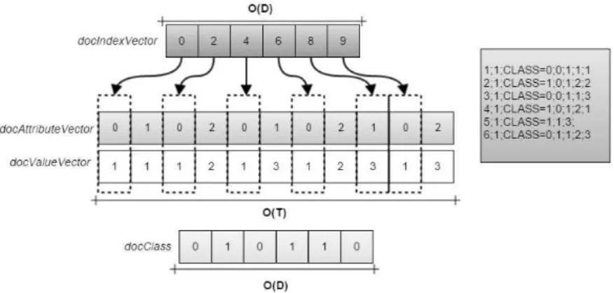
Given that document collections are usually sparse, with terms occurring only in a few documents, we chose to represent the documents by a compact data structure, based on inverted index. For this, we used four vectors: docIndexV ector represent-ing the documents; docAttributeV ector that stores the attributes of each document; docV alueV ector that stores the weights of the attributes for each document; and fi-nally,docClass that stores the classes of all documents. AtdocIndexV ectorthe index represents the document, and in each position of this vector we store the position where the list of terms of the document begins in vector docAttributeV ector and the frequency in the vector docV alueV ector. At docClass each index also represents a document, and each position stores the respective document class.

Figure 5.1 shows an example of the data structure used. As can be seen, the document 0 of the database, starts its list of terms at the index 0 of the vector docAttributeV ector and has two terms (terms 0 and 1), each of which has frequency equal to1as can be seen in vectordocV alueV ector. In turn, the document4begins its list of terms in the position 8 of the vectors docAttributeV ector and docV alueV ector and has only the term1, with frequency also equal to 3. The document classes are in the vectordocClass, where the documents0 and 4 have classes 0 and 1respectively.

Explorando estratégias bayesianas eficientes e eficazes para classificação de texto

EXPLORANDO ESTRATÉGIAS BAYESIANAS

EFICIENTES E EFICAZES PARA

FELIPE A. RESENDE VIEGAS

EXPLORANDO ESTRATÉGIAS BAYESIANAS

EFICIENTES E EFICAZES PARA

CLASSIFICAÇÃO DE TEXTO

Orientador: Marcos André Gonçalves

Coorientador: Leonardo Chaves Dutra da Rocha

Belo Horizonte

FELIPE A. RESENDE VIEGAS

EXPLOITING EFFICIENT AND EFFECTIVE

BAYESIAN STRATEGIES FOR TEXT

CLASSIFICATION

Advisor: Marcos André Gonçalves

Co Advisor: Leonardo Chaves Dutra da Rocha

Belo Horizonte

Resumo

Abstract

List of Figures

List of Tables

Contents

Chapter 1

Introduction

1.1

Context and Motivation

1.2

Master Thesis Hypotheses

1.3

Work Description

1.4

Contributions

1.5

Roadmap

Chapter 2

Basic Concepts and Settings

2.1

Automated Document Classification

2.1.1

ADC Classifier

2.2

Evaluation Techniques

2.3

GPU and CUDA

Chapter 3

Related Work

3.1

Naive Bayes Limitations

3.2

Naive Bayes Strategies and Feature Weighting

3.3

Semi-Naive Bayes

3.4

GPU parallelization

3.5

Chapter Summary

Chapter 4

Combining Learning Models and

Feature Weighting Strategies

4.1

Naive Bayes Learning Models

4.1.1

“Traditional” Naive Bayes

4.1.2

Interpolated Naive Bayes

4.1.3

One versus All Naive Bayes

4.1.4

Complement Naive Bayes

4.2

Feature Weighting Strategies

4.2.1

Term Frequency

4.2.2

Product of the term and inverse document frequency

(tf-idf)

4.2.3

Relative Frequency

4.3

Experimental Evaluation