J. Aerosp. Technol. Manag. vol.3 número2

Isabel Lima Hidalgo

EMBRAER São José dos Campos/SP – Brazil isabel.lima@embraer.com.br

Airton Nabarrete*

Technological Institute of Aeronautics São José dos Campos/SP – Brazil nabarret@ita.br

Marcelo Santos,

EMBRAER São José dos Campos/SP – Brazil marcesantos@embraer.com.br,

*author forcorrespondence

Structure-borne transmissibility

evaluation through modeling

and analysis of aircraft vibration

dampers

Abstract: In the aircraft industry a great practical relevance is given to the extensive use of vibration dampers between fuselage and interior panels. The proper representation of these isolators in computer models is of vital importance for the accurate evaluation of the vibration transmission paths for interior noise prediction. In general, simplifi ed models are not able to predict the component performance at mid and high frequencies, since they do not take into account the natural frequencies of the damper. Experimental tests are carried out to evaluate the dynamic stiffness and the identifi cation of the material properties for a damper available in the market. Different approaches for its modeling are analyzed via FEA, resulting in distinct dynamic responses as function of frequency. The dynamic behavior, when the damper natural modes are considered jointly with the high modal density of the plate that represents the fuselage, required the averaging of results in the high frequency range. At this aim, the statistical energy analysis is then used to turn the comparison between models easier by considering the averaged energy parameters. From simulations, it is possible to conclude how the damper natural modes infl uence the dynamic response of aircraft interior panels for high frequencies.

Keywords: Vibration damper, Fuselage structures, Vibroacoustic, Dynamic stiffness, SEA.

INTRODUCTION

In the aircraft manufacturing, interior panels are fastened to the fuselage structure by means of mountings designed to permit the easy disassembly in the case of maintenance. These mountings should also minimize the vibration transmission between the internal panels and fuselage and they are frequently called vibration dampers. Conceptually, these isolators are resilient elements that have been applied to structures aiming at minimizing the vibration transmission (Beranek and Vér, 1992). In aircraft design, isolators or dampers are of great practical relevance by their extensive use between fuselage and interior panels for minimizing the structure-borne vibration. Their proper representation in computer models helps the engineer on obtaining the accurate evaluation for vibration transmission paths between fuselage and interior panel, and consequently, the interior noise prediction.

Commonly, vibration dampers are based on rubber materials, due to some mechanical properties, such as high damping, low stiffness, and high bearing capacity (Downey et al., 2001). As the dynamic behavior of the rubber changes with load and environment conditions, the characterization of employed materials plays an important

role in the performance prediction of dampers. The temperature is an important parameter to be considered during the damper characterization, since the rubber material at low temperatures tends to be stiffer and to have higher damping. In opposite sense, when tested at high temperatures, it tends to have low stiffness and damping. In addition, the rubber properties are also dependent to frequency and strain (Jones, 2001). Some instances of rubber materials applied for vibration control are the natural rubber, neoprene, and silicone.

Different calculations are used to evaluate the damper behavior. A classical method represents the set damper-structure as a mass-spring-damper system and it is useful at low frequency predictions (Nashif et al., 1985). Nevertheless, this representation does not include some real system features, such as material nonlinearity and the component dynamic behavior. These features, associated with the fact that an isolated structure does not behave as a rigid body, inl uence the damper attenuation at mid and high frequencies (Snowdon, 1979; Beranek and Vér, 1992; Weisbeck, 2006).

The dynamic behavior of dampers is considered in some published calculation methods. One of them, the four-pole method, described by Molloy (1957), incorporates dynamic characteristics of isolators and structure as frequency dependent through transfer matrices. As well Received: 03/05/11

Accepted: 14/06/11

reported by Snowdon (1979), Weisbeck (2006) and Weisbeck et al. (2009) the parameters used in this method are usually obtained experimentally. An alternative prediction method can assess the damper attenuation considering its dynamic behavior through a detailed i nite element model (Jones, 2001). This is a robust and well-established method to solve engineering problems related to solid structures (Bathe, 1996).

In this research, solid i nite elements are used to model one damper which is an assembly of metallic and rubber parts. Parameters regarding to geometry and material properties applied to the damper are detailed and investigated. A very rei ned mesh is employed to model one damper in order to achieve accurate modal frequencies and modes. The results from i nite element analysis (FEA) are compared to the ones obtained from an experimental modal test and the i nite element model is updated by i nding the material properties that adjust it in accordance with experimental results.

The dynamic analysis of the set fuselage-isolator-panel is the motivation for this work. The fuselage-isolator-panel structural system is modelled by the component mode synthesis (CMS), in order to test different coni gurations for the vibration dampers. For damped structures the analytical approach to CMS (Craig Jr., 1987) is used to solve for the component undamped modes and frequencies, to assemble those modes into the coupled model, and to supplement the resulting system with assumed modal damping. CMS is usually considered for the analysis of structures that are built-up of several components (Ewins, 2000).

The structure-borne transmissibility to interior panels and the consequent noise radiation are considered as signii cant until 10 kHz. However, when dealing with the high-frequency range, FEA brings concerns such as the large model size and dynamic properties with some uncertainty. As alternative to these issues, the traditional method of statistical energy analysis (SEA) (Lyon and DeJong, 1995), is considered. SEA represents a i eld of study in which statistical descriptions of a system are

employed in order to simplify the analysis of complicated structural-acoustic problems, especially in the high-frequency range. Searching for a solution to the entire frequency range, some authors have also considered the possibility of enriching a SEA model with information from FEA or measurements. One has proposed a coupled solution scheme considering the “stiff” components modelled with i nite elements and the “soft or l exible” ones modelled with SEA (Shorter and Langley, 2005). Using engineering experience or by performing a large number of subcomponent calculations one can investigate whether a specii c subsystem should be considered as ‘‘stiff’’ or ‘‘soft’’. In the present work, the i nite element model of the damper is considered as a substructure in the FEA approach and also as a subcomponent model to the SEA. A comparison of results for both analyses is commented for the entire frequency range.

FINITE ELEMENT MODELING

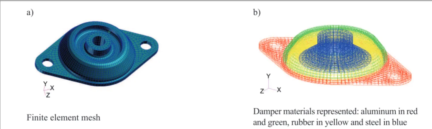
The i nite element model used in this research aims at discussing the inl uence of the high frequency vibration modes from damper and panels in the structure-borne transmissibility. A i nite element mesh very rei ned with solid elements is proposed for the isolator model, in order to achieve accurate modal frequencies and modes. Other models considering the vibration damper as a rigid connector or a spring is considered for comparison by the advantage of the simplii ed modeling. Figure 1(a) shows a rendered image of a damper available in the market with a rei ned solid mesh that contains at total 9,626 i nite elements (HEXA and PENTA) and 11,115 nodes. In Fig. 1(b), the same mesh appears with different colors for the material properties. The colors red and green represent the external structure made in aluminum; yellow and blue represent the component parts made in rubber and steel, respectively. The vibration damper selected to this work has the material properties described in Table 1. Also, as per the supplier catalogue (Lord Corporation, 2010), the modelled isolator has equivalent static stiffness equal to 88,000 N/m.

Figure 1. Isolator i nite element model

Y X Z

Y

X Z

Finite element mesh Damper materials represented: aluminum in red _{and green, rubber in yellow and steel in blue}

There are several possibilities to model the aircraft fuselage, but for this work just a simple uniform panel, or a rectangular aluminum plate, is used to represent the equivalent stiffness and mass distribution of a unit cell of fuselage. The same coni guration is used to the internal panel model. Fuselage and internal panels represented by uniform panels are modelled with plate i nite elements. The detail for the connection between meshes from the damper and panel is depicted in Fig. 2. The nodes of panel considered for the connection with the solid i nite element model of the damper are the same considered for other simulations, connecting the panels with the rigid or spring elements.

In this expression, d is the i nite element dimension, E is the Young modulus, ρ is the density, and f_lim is the mesh frequency limit. The lower wave speed leads to the lower mesh frequency limit, and it occurs for the rubber material. Hence, taking into account the rubber properties (Table 1) and an element dimension of 0.7 mm, the frequency limit for the current mesh is approximately 10 kHz.

Component mode synthesis

In CMS, the substructure or component models are transformed from physical to modal coordinates, using a set of normal modes after solving the component eigenvalue problem. The component models are assembled together to form the global dynamic problem for the entire structure. The equation of motion of a component r, neglecting damping, is described by Eq. 2, where the motion is represented by a vector of physical displacements. In this expression, written in a partitioned form, the indices j and i relate the vectors and matrices to boundary and internal nodes, respectively. M and K are the partitioned mass and stiffness matrices, while f represents the partitioned force vectors.



M_ii M_ij M_ji M_jj •

– ³ ³

— ˜ µ µ r

u_i u_j ¨ © « ª«

¬ ­ « ®« r

+ Kii Kij K_ji K_jj • – ³ ³

— ˜ µ µ r

u_i u_j ¨ © « ª«

¬ ­ « ®« r

= fi f_j ¨ © « ª«

¬ ­ « ®« r

(2)

In CMS with i xed interface, the response of a system is represented in terms of a set of ‘component’ modes and ‘constraint’ modes. The component modes are taken as a subset of the local modes when the boundary degrees of freedom are clamped. The constraint modes are given by the static response of the substructure when a unit displacement or rotation is applied to a given boundary degree of freedom while all other boundary degrees of freedom remain i xed (Craig Jr., 1981). The normal modes with i xed-interface represent the component modes in this work. The size of this eigenvalue problem equals the number of internal degrees of freedom. Each component model is transformed from physical to modal coordinates, using a set of normal modes.

Part Material Density

(kg/m³)

Poisson

coefi cient Loss factor (%)

Young modulus [Pa]

Damper external structure Aluminum 2,700 0.33 1 7.1 x 1010

Damper central i xture Steel 304 SS 8,300* _{0.28 1 2.0 x 10}11

Damper rubber Silicone 1,200 0.40 20 2.5 x 106

Fuselage and internal plates Aluminum 2,700 0.33 1 7.1 x 1010

* _{density to updated isolator mass.}

Table 1. Damper, fuselage and internal panel material properties

Figure 2. FEM model detail: isolator-plate interface

The panels are modelled, each of them as a substructure, with QUAD4 elements. The modal analysis of each one is performed by Nastran solver (MSC Software, 2008). The isolator mesh with solid i nite elements is dei ned in order to guarantee the minimum number to correctly represent the vibration modes. As a minimum amount recommended by Fahy and Gardonio (2007), six elements per wavelength are applied to the isolator mesh. The calculation of the wavelength λ is based on the propagation speed c_l of the quasi-longitudinal wave on solid, and evaluated as presented in Eq. 1.

6d =h= cf

f_lim = E /l

The reduction in the model size is achieved by truncating the number of component modes included in the analysis (Craig and Bampton, 1968). In CMS with ixed-interface, the modal matrix is formed by the combination of the kept number of normal modes with ixed-interface and the static constraint modes for the component. The constraint modes assure the compatibility of the component displacements at the interfaces, improve convergence and also yield the exact static solution. Equation 3 shows the relation between the physical coordinates and modal coordinates for the component model. In this equation, Φik and qk represent, respectively, the

kept normal modes and the modal coordinates with ixed-interface. The constraint coordinates are represented by q_c and I_jj is an identity matrix.

u_i u_j ¨ © « ª« ¬ ­ « ®« r

= \ik -Kii -1

K_ij

0 I_jj

• – ³ ³ ³ — ˜ µ µ µ r q_k q_c ¨ © « ª« ¬ ­ « ®« r (3)

The equation of motion based in modal coordinates of the component r is then presented in Eq. 4. The matrices m_cc and k_cc are the constraint modal mass and stiffness respectively, m_kc is the coupling matrix and Λ_kk is a diagonal matrix of kept modal eigenvalues.



I_ii m_kc m_kcT

m_cc • –

³

µ

+ Rkk 0 0 k cc • – ³ ³ — ˜ µ µ r q_k q c ¨ © « ª « ¬ ­ « ® « r = F 0 • –

³

—

µ

F_ik -K_ii-1K_ij 0 I_jj

rT f i f j r (4)

Considering the synthesis of two or more components and the continuity of the modal displacements at their common interface, a transformation matrix is written to impose the coupling conditions among them (Craig Jr., 1987). Due to the simplicity of the transformation matrix, the component synthesis is straightforward and the system matrices have the same structure as the component matrices.

Rubber material properties identiication

The rubber material is of great importance for the analysis of the isolator model, and in the present research, the rubber property identiication is based on dynamic stiffness measurements and later in the numerical adjustment.

The test procedure developed by Clark and Hain (1996) for measuring the axial dynamic stiffness is applied to the selected

vibration damper. It is axially excited by the shaker at one end while the other end is completely ixed, approximating to the one-degree-of-freedom experiment. The ratio between acceleration and applied force is taken as test result.



k= m -F

x

( )

2

(5)

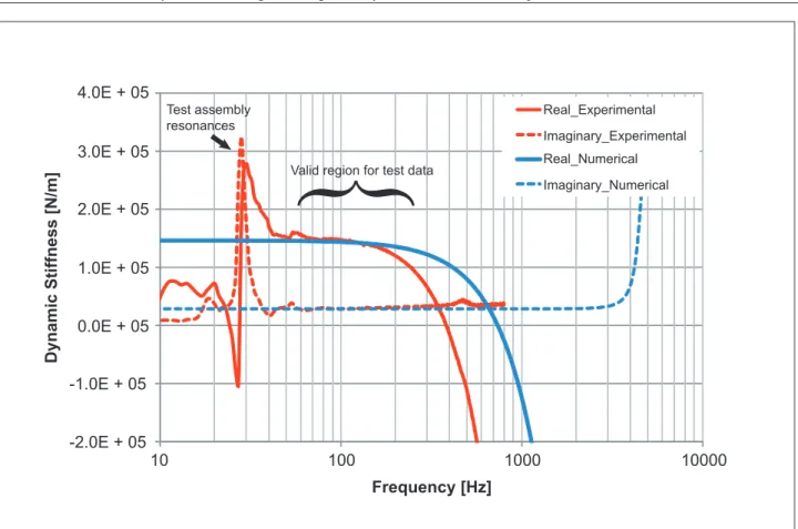
The dynamic stiffness k from the tested vibration damper is calculated by the Eq. 5. In that, f is the frequency and m is the mass from the moving parts of damper and the attached set, such as bolt and other parts. By the dimensions of the damper, the rubber material is considered as massless. The experimental result from this test is presented on Fig. 3. The irst peak is associated to test set. The test data is considered valid where the dynamic stiffness is constant. Above this value the response becomes very large since it is controlled by inertia, explaining the decrease in stiffness. From this test, the real part value of dynamic stiffness is 1.50x105 _{N/m, and the imaginary part value is}

2.89x104_{N/m. Calculated as the quotient of the imaginary}

part by the real part, the loss factor is approximately 0.2. Afterwards, frequency response analyses are employed as the identiication process for the isolator FE model, in order to it the experimental data.

Frequency-constant properties are used for the damper rubber material. Although the rubber properties are dependent on frequency, for typical applications of the damper studied in the current work, it is possible to consider a constant Young Modulus value since the damper elastomeric material is designed to work in the viscoelastic rubbery region.

In addition, dynamic analyses consider the unitary axial concentrated force applied on the damper central ixture. Concentrated mass is not considered, which differs from the experiment, and generates the later decreasing in real dynamic stiffness. Also, no perturbation at low frequency is observed in the numerical analysis. Finally, the updated Young Modulus of 2.5 MPa and loss factor of 20%, resulted in the best dynamic stiffness curve adjustment, as can be veriied in Fig. 3.

DAMPER DYNAMIC ANALYSIS

Frequency [Hz]

D

y

n

a

m

ic

Sti

ffn

e

s

s

[N

/m

]

10 -2.0E + 05 -1.0E + 05 0.0E + 05 1.0E + 05 2.0E + 05 3.0E + 05 4.0E + 05

100 1000

Real_Experimental Test assembly

resonances

Valid region for test data Real_Numerical Imaginary_Numerical Imaginary_Experimental

10000

{

Figure 3. Comparison between numerical (FEA) and experimental dynamic stiffness

Figure 4. Spring-Mass Modes

Mode 1. Radial mode 512.8 Hz

Mode 4. Torsion mode

755.3 Hz Mode 5. Rocking mode _{1138.1 Hz} Mode 2. Radial mode

514.7 Hz

Mode 6. Rocking mode 1148.9 Hz Mode 3. Axial mode

738.0 Hz

Y X Z

Y X Z

Y X Z

Y X Z Y

X Z Y

is seen in Fig. 4 and, how told by Gardner et al. (2005), these modes are described as spring modes. Also, it is possible to observe the symmetrical radial modes as a consequence of the geometry in this specii c damper.

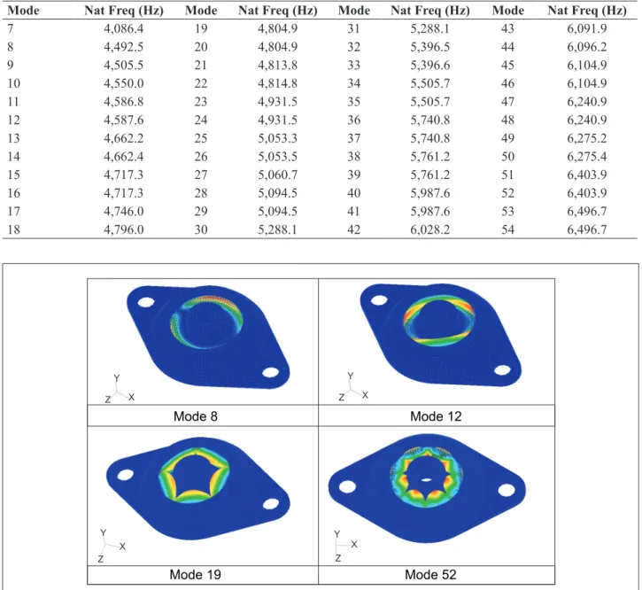
The modes that follow the spring modes are called rubber modes, in which this part of the damper responds for higher frequencies. For these vibration modes, the external metallic structure and the central i xture do not inl uence the natural damper motion. In the current case, these modes occur at very high frequency, from 4000 Hz and on, where each one is very close to the other in frequency. Table 2 describes the rubber modes until 6500 Hz. Figure 5 shows some of these rubber mode shapes.

FUSELAGE-ISOLATOR-PANEL ANALYSES The complexity of modeling the internal panels connected to the fuselage of an aircraft is evaluated by considering, as i rst model, two rectangular plates centrally connected by a vibration damper. This model recalls the concept of fuselage-isolator-panel, where one damper supports the internal panel attached to the fuselage. Then, two identical aluminum plates with thickness equal to 2 mm and dimensions equal to 0.5 m and 0.7 m are modelled with QUAD4 i nite elements. The material properties selected to this model are described on Table 1. The plates are separated by the damper height or approximately 8.25 mm. The rotation degree of freedom around each plate edge is restricted aiming at simulating the fuselage continuity.

Mode Nat Freq (Hz) Mode Nat Freq (Hz) Mode Nat Freq (Hz) Mode Nat Freq (Hz)

7 4,086.4 19 4,804.9 31 5,288.1 43 6,091.9

8 4,492.5 20 4,804.9 32 5,396.5 44 6,096.2

9 4,505.5 21 4,813.8 33 5,396.6 45 6,104.9

10 4,550.0 22 4,814.8 34 5,505.7 46 6,104.9

11 4,586.8 23 4,931.5 35 5,505.7 47 6,240.9

12 4,587.6 24 4,931.5 36 5,740.8 48 6,240.9

13 4,662.2 25 5,053.3 37 5,740.8 49 6,275.2

14 4,662.4 26 5,053.5 38 5,761.2 50 6,275.4

15 4,717.3 27 5,060.7 39 5,761.2 51 6,403.9

16 4,717.3 28 5,094.5 40 5,987.6 52 6,403.9

17 4,746.0 29 5,094.5 41 5,987.6 53 6,496.7

18 4,796.0 30 5,288.1 42 6,028.2 54 6,496.7

Table 2. Rubber material modes of the damper

Figure 5. Instances of rubber material mode shapes

Mode 19

Mode 8 Mode 12

Mode 52 Y

X Z

Y

X Z

Y X Z Y

Modal frequency responses using the substructure modal solutions are obtained for the entire structure considering different approaches for the isolators. Justii ed by the necessary simplii cation, distinct connection elements can be modelled between both plates, when dealing with the complete aircraft structure. Aiming at the response comparison, in this research, i ve approaches for isolators are modelled to connect both plates at the center, as follows:

1. rigid connection: The damper ini nite stiffness is used as reference to this approach;

2. linear axial spring connection: The damper static stiffness value of 88,000 N/m (Lord Coorporation, 2010) is considered as the constant dynamic stiffness;

3. linear axial spring connection: The dynamic stiffness value considered here is equal to 148,000 N/m, which is obtained from the test described in section 2.2, for the axial direction of the damper;

4. six degrees-of-freedom spring connection: The dynamic stiffness value per degree of freedom is considered as presented on Table 3. These values are obtained from other experiments performed in similar manner as described in section 2.2;

5. updated FE solid model for the damper, as described in the previous sections. The damper connection to the upper and bottom plates is performed through rigid elements. Figure 2 shows the rendered image for this connection.

In these analyses, the excitation force ranges in frequency from 1 to 8,000 Hz. Initially, only one concentrated harmonic force is applied perpendicular to the bottom panel. Subsequently it is proposed to create an average spectrum for each response. This is performed by applying six different excitations arbitrarily distributed and applied not simultaneously, as sketched in Fig. 6.

Hence, the dynamic response of the upper panel is obtained by averaging velocity in space considering chosen nodes, and afterward by averaging these results for the six different excitations. This data is calculated for each isolator approach. The velocity magnitude is considered as the response parameter, since it characterizes the vibration level.

FUSELAGE-ISOLATOR-PANEL SIMULATION RESULTS

After identifying the damper properties through experimental tests, the update is performed to the FE solid model. Then, the simulation result with this model is considered as the most accurate to represent the real damper behavior.

Figure 7 brings the low frequency results (1 to 100 Hz) in narrow band when only one excitation is applied. In this range, the behavior of the six-dof spring approach is the closer to the updated FE solid model. Signii cant differences among models can be noted in the anti-resonance behavior, when analyzing both axial spring models around 60 Hz, while other models show a resonance at 60 Hz. This fact indicates that this mode is related to the coupling with other directions, different from the axial one.

Direction Dynamic stiffness

(N/m) Loss factor η

X 1.0E+05 0.18

Y 1.0E+05 0.18

Z 1.5E+05 0.20

RX 2.8E+01 0.20

RY 2.8E+01 0.20

RZ 2.7E+01 0.14

Table 3. Dynamic stiffness and loss factor

Figure 6. FEM model sketch: response nodes positions and excitation points

Response nodes on the upper plate

Excitation Force on the bottom plate

Concentrate force at coordenates (0.126, 0.124, 0.0)

Connection between plates

F z

y

Figure 7.Upper plate velocity average in low frequency range (10 to 100 Hz)

1.0E + 00

1.0E - 01

1.0E - 02

1.0E - 03

1.0E - 04

1.0E - 05

1.0E - 06

10 Frequency [Hz]

|V

e

lo

c

ity

|

(m

/s

)

100 Rigid

Axial spring k = 88e3N/m

6 DOF spring

Updated FE solid model Axial spring k = 148e3N/m

Due to the high modal density of the plate at high frequency, the inl uence of rubber modes of the damper on the plate response may not be properly assessed. This fact justii es the need of an average spectrum for each response. The average spectrum is calculated for each isolator approach and presented in Fig. 8, considering frequency band of one-third octave from 100 to 6,300.

Based on Fig. 8, it is possible to notice a similar behavior for all models until 800 Hz, except for a decrease for the updated FE isolator model in 500 Hz. The rigid connection and the six-dof spring model follow similar trend along the entire frequency range, showing high vibration levels at high frequency when compared to the other models. Conversely the updated FE model shows that vibration level decreases with frequency from 1,000 Hz and on, such as both axial spring models. A difference however appears in the 4,000 Hz frequency band, where a vibration level increase is verii ed.

Facing the different approaches for isolator model, it is visible they result in distinct responses depending on the frequency of concern. Therefore, the simplicity of modeling the damper as axial springs when compared to the updated FE model is a worthy discussion. This is true since they show responses comparable to the

FE model for a proper frequency range. Although, in the high frequency range, the axial spring with the measured dynamic stiffness shows the same trend and values comparable to the updated FE model response, the difference related to the damper rubber modes can overestimate the damper attenuation.

Figure 8. Upper plate velocity magnitude (1/3 octave frequency band)

1.0E + 00

1.0E - 01

1.0E - 02

1.0E - 03

100 1000

1.0E - 04

Frequency [Hz]

|V

e

lo

c

ity

|

(m

/s

)

Rigid

Axial spring k = 88e3N/m

6 DOF spring

Updated FE solid model Axial spring k = 148e3N/m

COMPARISON BETWEEN FEA AND SEA

As presented in the previous section, simplii ed models for dampers are not feasible for predicting the high frequency vibration transmission. In this frequency range, although FEA can be employed, its results bring a complex task in interpreting the inl uence of isolator modes, due to the high modal density of the plate, requiring the need for averaging the results.

At the same time, the effort required to dei ne an FE model increases with size and with the geometric and material complexity of the model. Thus in order to obtain the response of complex structures, coupled through dampers, the use of FEA can be cost prohibited due to the high level of discretization required for the high frequency range. This issue for large models can be lessened by applying techniques such as component modal synthesis as described previously. However, in addition, there is uncertainty related to the dynamic properties of complex structures, regarding, for instance, the damping distribution, joints and connections between components, or the material properties. Consequently, it is granted that natural modes at high-frequencies based on a deterministic model with nominal material properties and dimensions may vary with real values and, as result, some statistical evaluation is required. FEA using Monte Carlo numerical simulation performs such analysis by repeating calculations for randomly generated sets of system

properties, which is, for high frequencies, a simulation with much time consuming. Also, excitation forces are not usually precisely known (Langley and Fahy, 2004).

As an alternative for vibroacoustic problems in the high frequency range, SEA is largely used, including in the aerospace industry (Lyon and DeJong, 1995). SEA allows the calculation of the l ow and storage of dynamic energy in a system. In SEA, a system is divided into subsystems, which are groups of similar energy storage modes. Each mode type in a SEA subsystem acts as a separate store of vibroacoustic energy and is therefore represented by a separate degree of freedom in the SEA equations. For each subsystem, as showed by Eq. 6, the energy dissipated internally (P_i,diss) by damping is proportional to the subsystem vibrational energy E_i. The proportionality rate is given by the internal loss factor

ηii, which can result from structural damping (material

property), acoustic radiation, subsystem interface, or friction mechanisms.

P_i,diss=M_ii\E_i

(6)

coupling loss factor (CLF) between system i and j. CLF depends on the characteristics of the junction between the subsystems and damping (Lyon and DeJong, 1995).

P_ij= t (d_ijE_i- d_jiE_j), n_id_ij= n_jd_ji

(7)

Equation 8 considers P_i as the power injected into the system, by the conservation of energy for n subsystems. There, the power losses, resulted from the dissipation (P_i,diss ) and the coupling (P_i→j ) of the subsystem, is diminished from the power gains (P_j→i ), coming from the coupled subsystems.

P_i= P_i,diss+ P_iAj

ji n

-

ji n

-(8)

Equations 7 and 8, in a matrix form, is written in Eq. 9. In this equation, [η0_{] represents the total loss factor matrix of}

the system deined by the internal and coupling loss factors, which are represented individually in Eq. 10. Finally, in Eq. 11, the power input P_i , due to a point structural source, considers force and velocity at the excitation point (Lyon and DeJong, 1995).

t u[d0

]{E}={P}

(9)

dij 0

= -dji , dii 0

= dim m =1

n

-(10)

P

i=

1

2Re Fuv

*

•– —˜

(11)

In SEA, the local modes of a subsystem are described statistically and the average response of the subsystem is predicted with respect to frequency and space (Lyon and DeJong, 1995). Since average parameters are considered, it is not necessary to have a detailed model. On the contrary, it is only required the overall length, width or volume of a subsystem along with approximate estimate of properties that govern the wave propagation within the subsystem. The response energy, from the model solution, is usually related to a particular quantity of interest such as acceleration, velocity, or sound pressure level.

The number of modes within a subsystem represents the capacity of the storage energy, hence the modal density characterizes the energy storage, and then, it is a restrictive parameter for SEA. The modal density of the isolator is low along the frequency range of interest, when compared to a typical subsystem in SEA, such as the rectangular plate. This fact restrains the capability of equivalent energy storage for proper calculation of the subsystem

parameters. The connection between subsystems is considered where impedance discontinuities exist. The measure of the energy rate lowing out of a subsystem through the coupling to another subsystem deines the CLF (Lyon and DeJong, 1995). Usually, within SEA models, the damper is represented by a CLF, since so far, there is not a speciic formulation for an isolator subsystem in SEA.

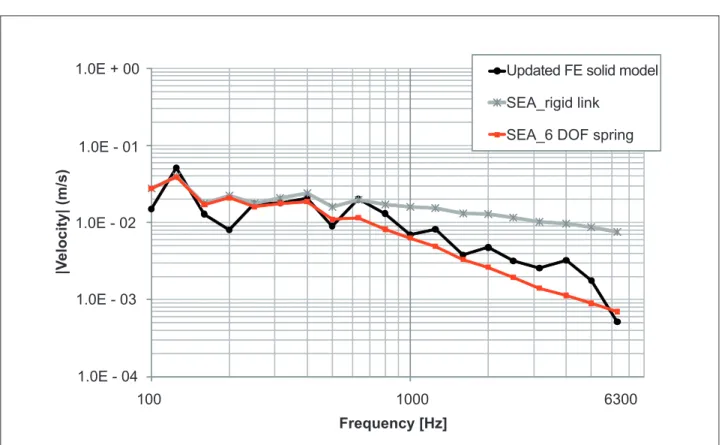
The comparison between FEA and SEA is achieved by modeling in SEA the same two simple panels connected by an isolator at the center point, as depicted in Fig. 6. SEA is performed using the software VaOne (ESI Group, 2009). In this software, two distinct connections are possible to choose for this comparison, the irst one with a rigid link, and the second one with a six-dof spring. For the last, it is considered the same dynamic stiffness values per direction given by Table 3. The power input in SEA model is calculated by Eq. 11, with the same driving point velocity adopted by FEA. In SEA, the power input is based on the average response resulting from six concentrated and harmonic forces, randomly distributed and applied not simultaneously. As required for comparison with SEA, the inite element response is obtained from the spatial average of velocity (using nine nodes), which is subsequently averaged for six different excitations. The comparison between FEA and SEA is depicted in Fig. 9. It shows similar behavior for all data up to 630 Hz. In the high frequency range, updated FE solid model has the same trend of the SEA model with the spring connection. However, the updated FE model presents that vibration level increase in the 4000 Hz frequency band, what coincides with the band where the rubber modes of the damper are concentrated. Hence, in order to not overestimate the damper performance in the high frequency, it is recommended to include the damper dynamic behavior into the SEA model.

1.0E + 00

1.0E - 01

1.0E - 02

1.0E - 03

100 1000 6300

1.0E - 04

Frequency [Hz]

|V

e

lo

c

ity

|

(m

/s

)

SEA_rigid link

SEA_6 DOF spring Updated FE solid model

Figure 9. Upper plate velocity magnitude from SEA model and update solid FE model

CONCLUSIONS

Within this paper the FE model of a typical vibration damper applied to the aircraft fuselage is developed. Based on this model, it is possible to identify the damper dynamic behavior: spring modes, and the rubber internal modes.

Different modeling forms of damper are applied between two plates. The result comparison demonstrates that simplii ed models, such as axial spring, can be easily and well employed depending on the frequency range of interest. Although, in low frequency, some agreement is verii ed, in high frequency, the simplii ed model can not reach a satisfactory result when compared to the updated FE solid model.

On the other hand, in order to model the damper through i nite elements with i delity, the rubber material properties must be reliable and be available, what is frequently a challenger. The FE model development is time consuming, mainly due to the rei ned mesh, as required for the high frequency limit.

In order to highlight the differences between models, mainly in high frequency, where the plate modal density is high, FE results are averaged. They show a vibration increase due to the damper rubber modes. In addition, applying simplii ed models, SEA is performed for comparison.

The vibration transmission through the dampers is of great importance in aircraft applications such as noise radiation from interior panels. For high frequency, it requires a proper modeling of the component, taking into account its internal vibration modes.

REFERENCES

Bathe, K. J., 1996, Finite element procedures, Prentice-Hall, New Jersey, USA.

Beranek, L. L., Vér, I. L., 1992, Noise and vibration control engineering - principles and application, Jonh Wiley & Sons Inc., New Jersey, USA.

Clark, M. D., Hain, H. L., 1996, A systematic approach used to design l oor panel isolation for commercial aircraft, Proceedings of Noise-Con 96, Seattle, USA, pp. 455-460.

Craig Jr., R. R., 1981, Structural dynamics, an introduction to computer methods, Wiley, New York.

Craig, R. R., Bampton Jr., M., 1968, Coupling of substructures for dynamic analysis, AIAA Journal 6, pp. 1313-1319.

Journal of Analytical and Experimental Modal Analysis, Vol. 2, pp. 59-72.

Downey, P., Bachman, G., Diffendall, C., 2001, Microcellular resilience for optimised insertion loss using an rubber insulating material, Proceedings of Noise-Con 2001, Portland, USA.

ESI Group, 2009, VaOne 2009 Guide.

Ewins, D. J., 2000, Modal testing: theory, practice and application, 2nd _{edition, John Wiley & Sons Inc., New}

York.

Fahy, F., Gardonio, P., 2007, Sound and structural vibration, 2nd edition, Elsevier, Oxford, UK.

Gardner, B. K., Shorter, P. J., Cotoni, V., 2005, Modeling vibration isolators at mid and high frequency using Hybrid FE-SEA Analysis, Proceedings of InterNoise 2005, Rio de Janeiro, Brazil.

Langley, R. S., Bremner, P. G, 1999, A hybrid method for the vibration analysis of complex structural-acoustic systems, Journal of the Acoustical Society of America, 105, pp.1657-1671.

Langley, R. S., Fahy F. J., 2004, Noise and Vibration, 1st

edition, Chapter 11 - Advanced Applications in Acoustics, Spon Press, London UK.

Jones, D. I. G., 2001, Handbook of viscoelastic vibration damping, Jonh Wiley & Sons Inc., West Sussex, England.

Lyon, R. H., DeJong, R. G., 1995, Theory and application of statistical energy analysis, Butterworth-Heinemann, Boston, EUA.

Lord Corporation, <http://www.lord.com>, in June 6, 2010.

Molloy, C. T., 1957, Use of four-pole parameters in vibration calculations, Journal of the Acoustical Society of America, Vol. 29, pp. 842-853.

MSC Software, 2008, MSC Nastran 2008 Quick Reference Guide.

Nashif, A. D., Jones, D. I., Henderson, J. P., 1985, Vibration damping, John Wiley & Sons Inc., New York, USA.

Shorter, P. J., Langley, R. S., 2005, Vibro-acoustic analysis of complex systems, Journal of Sound and Vibration, Vol. 288, pp. 669-699.

Snowdon, J. C., 1979, Vibration isolation: use and characterization, Journal of the Acoustical Society of America, Vol. 66, pp. 1245-1274.

Weisbeck, J. N., 2006, Effect of stiffness, damping, and design on side panel isolator noise attenuation characteristics, Proceedings of InterNoise 2006, Honolulu, USA.