CENTRO DE TECNOLOGIA
DEPARTAMENTO DE ENGENHARIA DE TELEINFORMÁTICA
PROGRAMA DE PÓS-GRADUAÇÃO EM ENGENHARIA DE TELEINFORMÁTICA MESTRADO ACADÊMICO EM ENGENHARIA DE TELEINFORMÁTICA
BRUNO SOKAL
SEMI-BLIND RECEIVERS FOR MULTI-RELAYING MIMO SYSTEMS USING RANK-ONE TENSOR FACTORIZATIONS
SEMI-BLIND RECEIVERS FOR MULTI-RELAYING MIMO SYSTEMS USING RANK-ONE TENSOR FACTORIZATIONS
Dissertação apresentada ao Curso de Mestrado Acadêmico em Engenharia de Teleinformática do Programa de Pós-Graduação em Engenharia de Teleinformática do Centro de Tecnologia da Universidade Federal do Ceará, como requisito parcial à obtenção do título de mestre em Engenharia de Teleinformática. Área de Concentração: Sinais e Sistemas
Orientador: Prof. Dr. André Lima Férrer de Almeida
Biblioteca Universitária
Gerada automaticamente pelo módulo Catalog, mediante os dados fornecidos pelo(a) autor(a)
S1s Sokal, Bruno.
Semi-Blind Receivers for Multi-Relaying MIMO Systems Using Rank-One Tensor Factorizations / Bruno Sokal. – 2017.
85 f. : il. color.
Dissertação (mestrado) – Universidade Federal do Ceará, Centro de Tecnologia, Programa de Pós-Graduação em Engenharia de Teleinformática, Fortaleza, 2017. Orientação: Prof. Dr. André Lima Férrer de Almeida.
1. MIMO systems. 2. cooperative communications. 3. semi-blind receivers. 4. rank-one tensors. I. Título.
SEMI-BLIND RECEIVERS FOR MULTI-RELAYING MIMO SYSTEMS USING RANK-ONE TENSOR FACTORIZATIONS
Dissertation presented to the Master Program in Teleinformatics Engineering at the Federal University of Ceará, as part of the requirements for obtaining the Master’s Degree in Teleinfor-matics Engineering. Concentration area: Signal and Systems.
Approved in: 27/07/2017.
EXAMINATION BOARD
Prof. Dr. André Lima Férrer de Almeida (Advisor) Federal University of Ceará
Prof. Dr. Carlos Alexandre Rolim Fernandes Federal University of Ceará
Prof. Dr. Walter da Cruz Freitas Junior Federal University of Ceará
I would like to express my deepest thanks to my mother, who has always encoura-ged me in the difficult moments of this journey. To my dad, who helped me build one of the contributions of this thesis, the generalization of the Kronecker approximation, and taught me to be more patient, and I would like to thanks to my brothers, Henrique, Junior and Waleska. Special thanks to Camila, for being patient with me and for the support during this period. To Prof. André, whom I also consider as a friend, for inspiring me as a person and as a scientist, and for all the patience he had with me during this journey (I know it must have been a lot). To FUNCAP, for the financial support.
Fortaleza, July 2017.
Cooperative communications have shown to be an alternative to combat the impairments of signal propagation in wireless communications, such as path loss and shadowing, creating a virtual array of antennas for the source. In this work, we start with a two-hop MIMO system using a a single relay. By adding a space-time filtering step at the receiver, we propose a rank-one tensor factorization model for the resulting signal. Exploiting this model, two semi-blind receivers for joint symbol and channel estimation are derived: i) an iterative receiver based on the trilinear alternating least squares (Tri-ALS) algorithm and ii) a closed-form receiver based on the truncated higher order SVD (T-HOSVD). For this system, we also propose a space-time coding tensor having a PARAFAC decomposition structure, which gives more flexibility to system design, while allowing an orthogonal coding. In the second part of this work, we present an extension of the rank-one factorization approach to a multi-relaying scenario anda closed-form semi-blind receiver based on coupled SVDs (C-SVD) is derived. The C-SVD receiver efficiently combines all the available cooperative links to enhance channel and symbol estimation performance, while enjoying a parallel implementation.
Comunicações cooperativas têm mostrado ser uma alternativa para combater os efeitos de propagação do sinal em comunicações sem-fio, como, por exemplo, a perda por percurso e sombreamento, criando um array virtual de antenas para a fonte transmissora. Neste trabalho, toma-se como ponto de partida um modelo de sistema MIMO de dois saltos com um único relay. Adicionando um estágio de filtragem no receptor, é proposta uma fatoração de posto unitário para o sinal resultante. A partir deste modelo, dois receptores semi-cegos para estimação conjunta de símbolo e canal são propostos: i) um receptor iterativo baseado no algoritmo trilinear de mínimos quadrados alternados (Tri-ALS) e ii) um receptor de solução fechada baseado na SVD de ordem superior truncada (T-HOSVD). Para este sistema, é também proposto um tensor de codificação espacial-temporal com uma estrutura PARAFAC, o que permite maior flexibilidade de design do sistema, além de uma codificação ortogonal. Na segunda parte deste trabalho, é apresentada uma extensão da fatoração de posto unitário para o cenário multi-relay e um receptor semi-cego de solução fechada baseado em SVDs acopladas (C-SVD) é desenvolvido. O receptor C-SVD combina de modo eficiente todos oslinkscooperativos disponíveis, melhorando o desempenho
da estimação de símbolos e de canal, além de oferecer uma implementação paralelizável.
Figure 1 – Three terminal system example . . . 15
Figure 2 – Three terminal MIMO system example . . . 16
Figure 3 – Illustration of a third-order tensorX . . . 20
Figure 4 – (a) Column fibers; (b) Row fibers; (c) Tube fibers . . . 21
Figure 5 – (a) Frontal slices; (b) Lateral slices; (c) Horizontal slices . . . 21
Figure 6 – Illustration of a third-order PARAFAC decomposition as the sum of the outer products of three vectors. . . 26
Figure 7 – Illustration of a Tucker decomposition. . . 30
Figure 8 – Illustration of a Tucker-(2,3) decomposition. . . 31
Figure 9 – Illustration of a Tucker-(1,3) decomposition. . . 32
Figure 10 – 3-D Illustration of aN-thorder Nested Tucker decomposition. . . 33
Figure 11 – 3-D illustration of a 4-thorder Nested Tucker tensor. . . 34
Figure 12 – 3-D illustration of a 5-thorder Nested Tucker tensor. . . 35
Figure 13 – System model. . . 46
Figure 14 – Rank-one decomposition of the filtered signal tensor. . . 51
Figure 15 – Coding gain of the Zero-Forcing with Perfect CSI knowledge. . . 58
Figure 16 – Symbol error rate performance vs. ES/No. . . 58
Figure 17 – NMSE for Source-Relay channel. . . 59
Figure 18 – NMSE for Relay-Destination channel. . . 59
Figure 19 – Number of FLOPS vs. MDreceiver antennas. . . 60
Figure 20 – Number of iterations for ALS’s algorithms to converge. . . 60
Figure 21 – MIMO multi-relaying system. . . 62
Figure 22 – First phase of the transmission. . . 63
Figure 23 – Second phase of the transmission. . . 64
Figure 24 – Third phase of the transmission. . . 65
Figure 25 – Fourth phase of the transmission. . . 66
Figure 26 – Perfect CSI performance for different values ofP,J andK. . . 77
Figure 27 – Performance of the proposed receiver with different number of phases and signals to couple. . . 77
Figure 28 – Normalized mean square error. . . 78
2LSKP 2 steps Least Square Kronecker Product ALS Alternating Least Squares
DS-CDMA Direct Sequence Code Division Multiple Access C-SVD Coupled SVD
CONFAC Constrained Factor decomposition
ES/No Energy per symbol to noise power spectral density ratio FLOPS Floating-point Operations Per Second
HOOI Higher-Order Orthogonal Iteration
HOSVD Higher-Order Singular Value Decomposition LS Least Squares
MIMO Multiple Inputs Multiple Outputs MRC Maximal Ratio Combining NMSE Normalized Mean Square Error
NTD(4) Fourth-Order Nested Tucker Decomposition NTD(5) Fifth-Order Nested Tucker Decomposition PARAFAC Parallel Factors
QAM Quadrature Amplitude Modulation SER Symbol Error Rate
SIC Self Interference Cancellation SNR Signal-to-Noise Ratio
SVD Singular Value Decomposition Tri-ALS Trilinear Alternating Least Squares TSTC Tensor Space-Time Coding
C Field of complex numbers
(·)H Hermitian operator (·)T Transpose operator vec(·) Vectorization operator
unvec(·) Inverse operation to vectorization
· ◦ · Outer product
· ⊗ · Kronecker product
· ⋄ · Khatri-Rao product
· ×n· n-mode product
· •m
n · Contraction operator
· ⊔N· Concatenation operator
|| · ||F Frobenius norm
k · k2 Euclidean norm
1 INTRODUCTION . . . 13
1.1 Relay Channels . . . 14
1.1.1 Cooperative Communications. . . 15
1.2 Contributions . . . 17
1.3 Thesis organization . . . 18
1.4 Scientific production . . . 19
2 TENSOR PREREQUISITES . . . 20
2.1 Tensors . . . 20
2.2 Tensor Decompositions . . . 26
2.2.1 PARAFAC Decomposition . . . 26
2.2.1.1 PARAFAC Slices . . . 27
2.2.1.2 n-mode unfolding . . . 27
2.2.1.3 Uniqueness . . . 28
2.2.1.4 ALS Algorithm . . . 28
2.2.2 Tucker Decomposition . . . 30
2.2.2.1 Uniqueness . . . 30
2.2.2.2 Special Tucker Decompositions . . . 31
2.2.2.3 Higher-Order Singular Value Decomposition (HOSVD) Algorithm . . . 32
2.2.3 Nested Tucker Decomposition . . . 33
2.2.3.1 Fourth-Order Nested Tucker Decompositions (NTD(4)) . . . 34
2.2.3.2 Fifth-Order Nested Tucker Decomposition (NTD(5)) . . . 35
2.3 Kronecker Product Approximation . . . 36
2.3.1 From Kronecker Approximation to Rank-one Matrix . . . 36
2.3.2 From Kronecker Product Approximation to Rank-one Tensor . . . 37
2.3.3 From Kronecker-Sum Approximation to Rank-R Tensors. . . 41
2.4 Khatri-Rao factorization of a DFT matrix . . . 42
2.5 Summary . . . 45
3 TWO-HOP MIMO RELAYING . . . 46
3.1 System Model . . . 46
3.1.1 Coding Tensor Structure . . . 48
3.2 Semi-Blind Receivers . . . 52
3.2.1 Tri-ALS receiver . . . 52
3.2.2 T-HOSVD receiver . . . 53
3.3 Computational Complexity . . . 55
3.4 Simulation Results . . . 55
3.4.1 Perfect CSI Channels . . . 56
3.4.2 Symbol Error Rate . . . 56
3.4.3 Normalized Mean Square Error . . . 56
3.4.4 FLOPS . . . 57
3.5 Summary . . . 61
4 MULTI-RELAYING MIMO SYSTEM . . . 62
4.1 System Model . . . 62
4.1.1 Destination Signals . . . 67
4.1.2 Coding Tensor Structure . . . 67
4.1.3 X(SR1D)Processing . . . 68
4.1.4 X(SR1R2D)Processing . . . . 69
4.1.5 Uniqueness . . . 71
4.2 C-SVD Receiver. . . 71
4.2.1 Similar Systems . . . 74
4.3 Simulation Results . . . 74
4.3.1 Symbol Error Rate . . . 75
4.3.2 Normalized Mean Square Error . . . 76
4.4 Summary . . . 79
5 CONCLUSION . . . 80
BIBLIOGRAPHY . . . 82
APPENDIX . . . 86
APPENDIX A – Coding Orthogonality Design . . . 86
1 INTRODUCTION
The use of multiple antennas at the transmitter side and receiver side brought new gains to wireless communications to exploit and new challenges compared with single antenna wireless systems. Among these gains, we highlight spatial diversity and spatial multiplexing gains. The spatial diversity gain comes from the use of multiple antennas to combat the fading in wireless communications. The spatial multiplexing gain comes from the transmission of multiple data streams in rich scattering environments, increasing the system spectral efficiency [1, 2, 3]. However, consider the case of a MIMO wireless system where the source has no line of sight with the destination or, the links between them are too poor. In this scenario, the use of relay stations has shown to be an alternative to combat fading and to increase the capacity and coverage of wireless system [4, 5, 6]. The benefits of relay-assisted wireless communications strongly rely on the accuracy of the CSI for all the links involved in the communication process. Moreover, the use of precoding techniques at the source and/or destination [7, 8] often requires the instantaneous CSI knowledge of all links. An example of a cooperative communication scenario is that of a multi-user system, where each user can be viewed as a relay station that assists the source.
Even thought, those users may have a single antenna only, the system exploits the spatial diversity as a MIMO system, due to the virtual antennas provided by the relay nodes. Some works in this application can be viewed in [9, 10, 11, 12]. In [9], the authors investigate a multi-user cooperative system with relay coding to enhance the performance of 4G systems. In [10] and [11], a multi-user cooperative system with AF protocol at the relay is studied. In[10], the authors focus on the problem in which scenario the relay must cooperate, and in [11], the authors proposed a multi-user detection for uplink DS-CDMA in a multi-relaying scenario taking advantage of the multidimensional nature of the signal, using tensor decompositions for parameter estimation. In [12], the authors investigate the problem of power allocation for a multi-user multi-relaying system with DF protocol in cognitive radio networks using bandwith-power product to reach a optimal spectrum-sharing. In the context of 5G systems, we can cite the recent work [13] where the authors proposed a non-orthogonal multiple access for downlink, where the system is divided in K time slots with K−1 users and each user
tensor algebra for wireless communications has been growing up, at most after the work of Sidiropoulos [14]. The main interest has been on the use of tensor decompositions to model the received signal as well as to derive receiver algorithms exploiting multiple forms of signal diversity. The two most common tensor decompositions are PARAFAC (Parallel Factor) [15] and Tucker [16] decompositions. Alternative tensor decompositions have been developped recently ([17, 18, 19, 20]). The PARAFAC decomposition is the most popular one, and not only for its conceptual simplicity but also for its uniqueness property [21]. The Tucker decomposition, is note unique in general. However, when the core tensor it is known, the factors are unique under some scalar ambiguity [17]. In the context of MIMO wireless communication, in [19, 20, 22] semi-blind receivers have been proposed to jointly estimate the channel and the symbols using tensors modeling.
In the cooperative scenario, some works that propose receivers based on the use of tensor modelling can be found in [23, 24, 18, 17]. The work [23] develops a tensor-based channel estimation algorithm for two-way MIMO relaying systems using training sequences. In [24], a supervised joint channel estimation algorithm is proposed for one-way three-hop communication systems with two relay layers. In [18], the authors proposed a semi-blind receiver for two-hop MIMO relaying systems using a Nested PARAFAC model. The authors in [17] developed first a generalization of the work [18], so called Nested Tucker decomposition, by using full tensors as space-time coding (random exponential structure), at the source and the relay. They also proposed two semi-blind receivers. The first one is an iterative solution based on the ALS (Alter-nating Least Squares), while the second is a closed-form solution based on LSKP (Least Squares Kronecker Product) factorization. The ALS receiver exploits the dimensions of the received signal to estimate symbol and channel matrices. However, this algorithm requires extensive matrix products and matrix inversions for each iteration. On the other hand, the Kronecker factorization receiver is suboptimal since it divides the relay-destination channel and symbol estimations into two steps (2LSKP), and the estimation for source-relay channel depends on the accuracy of the previous estimation.
1.1 Relay Channels
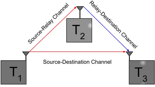
Figure 1 – Three terminal system example
T
1
T
2
T
3
Source-Relay Channel
Relay-Dest
inat ion
Channel
Source-Destination Channel
Source: Created by the Author
the data to destination (terminal 3), such cooperation divides the transmission into two phases, in the first, the terminal 1 sends the data to terminal 2 by a source-relay channel and to terminal 3 by a direct link, source-destination channel. Then, in the second phase, the terminal 2 sends to terminal 3 its own data plus the data from terminal 1 in the first phase. The system is illustrated in Figure 1, where the red line represents the transmission in the first phase and the blue in the second phase.
1.1.1 Cooperative Communications
In Figure 2 a three-terminal MIMO system is illustrated. This configuration combines the gains of MIMO systems and cooperative communications which can be summarized as
• Spatial Diversity
Figure 2 – Three terminal MIMO system example
T
1
T
3
T
2
T
2
Source-Relay Channel
Relay-Dest
inat ion
Channel
Source-Destination Channel
Source: Created by the Author
• Spatial Multiplexing
Considering the system in figure 2 the multiplexing gain is related to the gain of using multiple antennas for transmitting independent data streams (as discussed previously). The difference is that in this cooperative communication, the independent data streams are sent through the relay channels, leading to the next advantage.
• Coverage Area
As seen in Figure 2, the link between terminal 1 and terminal 2 and the link between terminal 2 and terminal 3 are shorter than the link between the terminal 1 and terminal 3, i.e. the path loss is smaller in the relay links than in the direct link, resulting in a less power for terminal 1 to reach terminal 3.
In terms of medium access, the relays usually are characterized as
• Full-Duplex
• Half-Duplex
In this configuration, the relay receives and transmits at different time slots. However, the latency of the system is increased, which in the case of a two-hop one relay system, the transmission rate has a drop of 50%. This configuration is the most common for relays, and appears in several works [17, 18, 28, 29].
In literature, there are many relay processing protocols that can be found in [4, 30, 31]. Basically, the protocols are divided into fixed relaying schemes and selective relaying schemes [4]. In a simple way, for the fixed relaying schemes the protocol used at the relay node is independent of the quality of the channel. The selective relaying schemes take into account the SNR of the received signal at the relay node. If the SNR exceeds a predefined threshold, the relay can apply the protocol. Else, the relay can remain idle. Next, we present some fixed relaying schemes protocols.
• Fixed Amplifying and Forward (AF)
Also known as a non-regenerative protocol, the relay receives the signal from the source and scales it. This protocol is attractive for systems that consider constant channels, due to simplicity and latency time. The use of the AF protocol makes more sense in the cases where the relay is closer to the destination than the source to compensate the fading. Otherwise, the relay has to use more power which also amplifies the noise in the received signal [6].
• Fixed Decode and Forward (DF)
Also known as a regenerative protocol, the DF consists of decoding the signal at the relay, then possibly applying some coding before forwarding to the destination. This scheme, compared with AF protocol, increases the latency of the system since some signal processing technique must be applied to decode the signal. For such protocol, it is useful that the relay is closer to the source than to the destination to have a better probability to decode the signal correctly than if the relay is closer to the destination [4, 6].
1.2 Contributions
The main contributions of this thesis can be summarized as
This process is a generalization of the Kronecker product approximation introduced by Van Loan in [32] that minimizes the Frobenius norm of a matrix by the Kronecker product of two matrices, rearranging the structure to a rank-one matrix. The proposed generalization rearranges the matrix structure into a tensor which can be approximated by the outer products ofN vectors, where those vectors are the vectorization of the original matrices
involved in the Kronecker product.
2. Orthogonal effective codes designed by the exact Khatri-Rao factorization of a DFT matrix. We show that a DFT of size K×K can be factorized into the Khatri-Rao product of N
matrices, with the constraint thatk1k2···kN =K, wherekn is the number of rows of the
n-thmatrix factor.
3. Two semi-blind receivers for two-hop MIMO cooperative systems are proposed by exploit-ing a rank-one tensor approximation. The first receiver is iterative (based on ALS), while the second is a closed-form solution (based on the HOSVD).
4. A coupled SVD-based semi-blind (C-SVD) for a multi-relaying MIMO system which provides closed-form estimates of the channels and symbols by coupling multiple SVDs.
1.3 Thesis organization
• Chapter 2 - Tensor Prerequisites
In this chapter, tensor arrays with some definitions and operations are introduced. The useful tensor decompositions for this thesis is presented. Also, an important topic is discussed, the generalization of the Kronecker approximation by Van Loan [32] which is the core part of the signal processing applied in the latest chapters and the DFT factorization by a Khatri-Rao product.
• Chapter 3 - Two-Hop MIMO Relaying
A two-hop MIMO relay system is presented, which is modelled using the decompositions introduced in Chapter 2, resulting into two semi-blind receivers. The first one is iterative while the second is based on a closed-form solution. Both receivers exploit the rank-one tensor formulation of the received signal after a space-time combining.
• Chapter 4 - Multi-Relaying MIMO System
rank-one tensors (one for each cooperative link) using the SVD.
• Chapter 5 - Conclusions
In this chapter, we draw the final comments and conclusions of this work, and highlight topics for future work.
1.4 Scientific production
Two papers have been produced as a result of this thesis. The first to a national congress of telecommunications and signal processing (SBrT 2017). The second paper has been submitted to the Journal of Communications and Information Systems, and we are waiting for the response.
1. Bruno Sokal, André L. F. de Almeida and Martin Haardt "Rank-One Tensor Modeling Approach to Joint Channel and Symbol Estimation in Two-Hop MIMO Relaying Systems
published in the XXXV Simpósio Brasileiro de Telecomunicações, São Pedro, Brazil, 2017 ;
2. Bruno Sokal, André L. F. de Almeida and Martin Haardt "Semi-Blind Coupled Receiver to Joint Symbol and Channel Estimation Using Rank-One Tensor Factorizations for MIMO
2 TENSOR PREREQUISITES
In this chapter, we start with the basis of tensor algebra, some properties and notations. In a second part, some useful decompositions that we make use in this thesis are presented. Finally, the generalized Kronecker approximation and the DFT factorization by a Khatri-Rao product are discussed.
2.1 Tensors
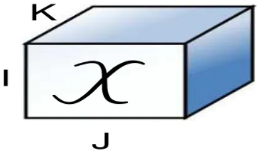
A tensor is an array with order greater than two (scalars have order zero, vectors order one, matrices order two), or simply a multidimensional array.
A tensorX ∈CI1×I2×···×IN is a multidimensional array with orderN, with elementsX
(i1,i2,···,in),
wherein={1···IN}. In the following, some definitions are presented. For a better understanding consider a third-order tensorX ∈CI×J×K.
Figure 3 – Illustration of a third-order tensorX
X
I
K
J
Source: Created by the Author
Definition 1. Fibers
Fibers are vectors formed by fixing the indices of all dimensions with the exception of one. For third-order tensors, there are three types of fibers: Column fibers, denoted byx.jk, where the indices for theJ andKdimensions are fixed and the indices of theI dimension is varying,
forming a vector of sizeI×1; Row fibers are denoted byxi.k, in this case the fixed dimensions areIandK, and the dimensionJis varying, resulting in a vector of sizeJ×1. At last, Tube fibers
are denoted byxi j.creating a vector of sizeK×1 by fixing the indices of theI andJ dimensions,
Figure 4 – (a) Column fibers; (b) Row fibers; (c) Tube fibers
(a) (b) (c)
Source: Created by the Author
Figure 5 – (a) Frontal slices; (b) Lateral slices; (c) Horizontal slices
(a) (b) (c)
Source: Created by the Author
Definition 2. Slices
Slices are formed by fixing one index and varying the others. For a third-order tensor X ∈
CI×J×K, slices are matrices and there are three different ways to slice it. Frontal slices are de-noted byX..kand are formed by varying the first and second modes and fixing the index along the third mode resulting inKmatrices of sizeI×J. Lateral slices are denoted byX.j., in this case the
index of theJdimension is fixed while the indices of the first and third modes are varying, at total
resulting inJmatrices of sizeI×K. The last one for third-order tensors are the Horizontal slices,
denoted byXi.., where now the index of the first mode is fixed and the indices of the second and third modes are now varying, yieldingImatrices of sizeJ×K. Figure 5 shows this representation.
Definition 3. n-mode unfolding
One way to matricizes a tensor is to compute the n-mode unfolding. Consider the tensor
X ∈CI×J×K, then-mode unfolding ofX is denoted byX(n)and this operation separates the n-th mode fibers and put them along the rows, resulting in the flatn-mode unfoldingX(n), or
SinceX it is a third-order tensor, there are three possible ways to matricize it. Let us denote
X(1)∈CI×JK,X(2)∈CJ×IK andX(3)∈CK×IJas the flat 1-mode, 2-mode and 3-mode unfolding ofX. The elements of then-mode unfoldingX(1)
(i,α),X(2)(j,β) andX(3)(k,γ) are mapped fromX as
α = j+ (k−1)J, (2.1)
β =i+ (k−1)I, (2.2)
γ =k+ (j−1)K, (2.3)
withi={1···I}, j={1···J},k={1···K},α ={1···JK},β ={1···IK}andγ ={1···IJ}.
This mapping is known as the little-endian convention, defined in [33]. For the general case of a N-th order tensor Y ∈CI1×···×IN, the element of the flat n-mode unfolding Y
(n)(in,l) ∈ CIn×I1···In−1In+1···IN is mapped fromY as
l=i1+ (i2−1)I1+ (i3−1)I1I2+···+ (iN−1)I1···In−1In+1···IN−1, (2.4)
wherein={1···In}andl={1···I1···I(n−1)I(n+1)···IN}.
Definition 4. Generalizedn-mode unfolding
Instead of separating one mode from the others, as in the n-mode unfolding, the generalized
n-mode unfolding matricizes the tensor by combining multiple modes as rows and columns of the
resulting unfolding matrix. Defining j={i1,···,in}andk={in+1,···,iN}within={1···In}, then-mode generalized unfolding maps the elements ofY(i
1,···,iN)into a matrixY[j,k]as
j=i1+ (i2−1)I1+ (i3−1)I1I2+···+ (in−1)I1I2···In−1 (2.5) k=in+1+ (in+2−1)In+1+···+ (iN−1)In+1In+2···IN−1 (2.6)
Definition 5. n-mode product
Given the third-order tensorX ∈CI×J×Kand a matrixA∈CR×I, then-mode product linearly combines the 1-mode fibers with the columns of the matrixAresulting a tensorYR×J×K. The n-mode product is denoted as
Y =X ×1A. (2.7)
This combination can be also expressed in terms of then-mode unfolding , i.e.
Then-mode product has the following property:
Y =X ×1A×1B×1C (2.9)
=X ×1CBA⇐⇒ (2.10)
Y(1)=CBAX(1). (2.11)
Definition 6. Contraction
This operation combines two tensors that have a common mode [34]. For example, given two third-order tensorsXI×J×K andYJ×L×M, whereJ is a common mode, the contraction between them is defined as
G =X •12Y, (2.12)
whereGI×K×L×M is a fourth-order tensor. The upper index in the operator "•" refers that the
contracted mode is, in this case, involves the first mode of the tensor at the right side and the lower index indicates the mode that will be contracted in the left side tensor. In element-wise, the tensorG can be written as
G(i,k,l,m)=
J
∑
j=1
X(i,j,k)Y(j,l,m) (2.13)
Definition 7. Concatenation
Consider the third-order tensor XI×J×K and the following matrices A(i) of size I×J, with i={1···R}. We can form a tensorGI×J×(K+R)as
G =X ⊔3A(1)⊔3A(1)⊔3··· ⊔3A(R). (2.14)
This operation concatenates all the matrices along the third dimensionK. In this case, the frontal
slices of tensorG are given by:
G..1:K =X..1:K (2.15)
G..K+1=A(1) (2.16) G..K+r=A
(r) (2.17)
G..K+R =A
Consider now a fourth-order tensorY ∈CI×J×K×L andRthird-order tensorsX(r)∈CI×K×L, we can concatenate all those R tensors into the second mode of the tensor Y, forming the
fourth-order tensorT ∈CI×(J+R)×K×L as:
T =Y ⊔2X(1)⊔2··· ⊔2X(R) (2.19)
The third-order tensors formed by fixing the second mode ofT are given as:
T.
1:J..=Y (2.20)
T.
J+1..=X
(1) (2.21)
T.
J+r..=X
(r) (2.22)
T.
J+R..=X
(R) (2.23)
Definition 8. Rank-one tensor
AN-thorder tensorYI1×···×IN is said to have a rank-one if we can writeY as the outer product
ofNvectors,
Y =a(1)◦ ··· ◦a(N), (2.24)
wherea(i)is a vector of sizeI
i×1, andi={1···N}.
Definition 9. Tensor rank
The typical rank of the tensorX is given by the smallest number of rank-one tensors yieldX
as linear combination. IfX has rankR, we have
X =
R
∑
r=1
ar◦br◦cr (2.25)
Definition 10. vec(·) operator Given a matrixA∈CI×J
A=
| ... |
a1 ··· aR
| ... |
I×R
, (2.26)
the vectorization ofAconsists of stacking the columns ofAas:
vec(A) =
a1
... aR
IR×1
The unvec(·)operator is the inverse operator of the vec(·).
Definition 11. Kronecker Product
Given a matrixAof sizeI×J and a matrixBof sizeR×S, the Kronecker productC=A⊗Bis defined as
C=
a11B a12B ··· a1JB
a21B a22B ··· a2JB ... ... ... ...
aI1B aI2B ··· aIJB
RI×SJ
(2.28)
Note that the matrixCcan be viewed as a block matrix withRblocks in the rows,Sblocks in
the columns and each block is a matrix of sizeI×J. Let us define some useful properties of this
product. For matricesA,B,CandDof compatible dimensions, we have:
(A⊗B)T=AT⊗BT (2.29) (A⊗B)∗=A∗⊗B∗ (2.30) (A⊗B)†=A†⊗B† (2.31) (A⊗B)(C⊗D) =AC⊗BD (2.32) vec(ABC) = (CT⊗A)vec(B) (2.33) vec(a(N)
◦ ··· ◦a(1)) =a(1)⊗ ··· ⊗a(N) (2.34)
Definition 12. Khatri-Rao Product
This product is also known as the column-wise Kronecker product. Given the matricesX∈CM×N, Y∈CL×N, the Khatri-Rao, defined asZ=X⋄Y, is given by
Z=h x1⊗y1 x2⊗y2 ··· xN⊗xN
i
LM×N (2.35)
wherexnandynare then-thcolumn of the matricesXandY,respectively. For matricesA,B,C andDof compatible dimensions, we have:
(A⊗B)(C⋄D) =AC⋄BD (2.36) vec(ADn(B)C) = (CT⋄A)bTn, (2.37)
2.2 Tensor Decompositions
We now present a few tensor decompositions that will be useful in the next chapters, namely the PARAFAC, Tucker and Nested Tucker decompositions. During the past decade, others decompositions were developed with applications in communication systems, such as: CONFAC [19], PARATUCK [20]. More recently, some generalized tensor decompositions have been developed such as the Tensor Train (TT) decomposition [35], Nested PARAFAC [18] and Nested Tucker [17].
2.2.1 PARAFAC Decomposition
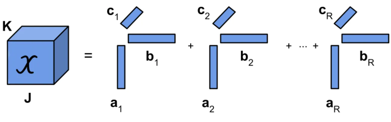
Figure 6 – Illustration of a third-order PARAFAC decomposition as the sum of the outer products of three vectors.
X
=
+ + ... +a
1a
2a
Rb
1b
2b
Rc
1c
2c
RI
J
K
Source: Created by the Author
The Parallel Factors (PARAFAC) decomposition, also known as Canonical Decom-position (CANDECOMP) [36] and Canonical Polyadic (CP) [37], is the most popular tensor decomposition. It factorizes aN-thorder tensor into a sum of the outer product ofN vectors. In
order to simplify, Figure 6 shows a PARAFAC decomposition of a third-order tensorXI×J×K,
A= | | ··· |
a1 a2 ··· aR
| | ··· |
I×R B= | | ··· |
b1 b2 ··· bR
| | ··· |
J×R
C= | | ··· |
c1 c2 ··· cR
| | ··· |
K×R
.
So we can writeX using a shorthand notation as
X =
R
∑
r=1
ar◦br◦cr (2.38)
= [[A,B,C]].
2.2.1.1 PARAFAC Slices
For a third-order PARAFAC tensor, its matrix slices can be represented as a function of its factor matrices. The frontal, horizontal and lateral slices can be respectively written as
X..k=ADk(C)BT (2.39) Xi..=CDi(A)BT (2.40) X.j.=ADj(B)CT (2.41)
2.2.1.2 n-mode unfolding
Considering now aN-thorder tensorXI1×···×IN of rankRand factor matricesA(i)
of sizeIi×R, withi={1···N}. The tensorX can be expressed in terms of then-mode product notation as
X =IR×1A(1)×2A(2)×3··· ×NA(N), (2.42)
whereIRis the superdiagonalN-thorder tensor of sizeR× ··· ×Rwith the entries equal to one,
if all indices are the same, and zero else. From Equation (2.42), the flatn-mode unfolding ofX
can be written as:
2.2.1.3 Uniqueness
One of the properties that makes PARAFAC such a popular tensor decomposition is uniqueness. Differing from matrix decompositions, such as SVD, where the pair of singular matrices is unique under the imposition of orthogonality, the uniqueness of the PARAFAC decomposition can be achieved by a far simpler condition. Uniqueness means that in Equation (2.38) the columns of the factor matrices can be arbitrarily permuted and scaled, so that
X = [[AΠ∆A,BΠ∆B,CΠ∆C]], (2.44)
whereΠ is some permutation matrix and ∆A,∆B,∆C are diagonal matrices containing the scaling factors, with∆A∆B∆C=IR, whereIR is the identity matrix of sizeR×R.
For third-order tensors, in 1977, Kruskal [21] derived a sufficient condition for uniqueness. This condition relies on the so-calledk-rank. If a matrix have ak-rank equal tol, it
means that every set ofl columns of this matrix is linearly independent. Denoting askA,kBand
kCas thek-rank ofA,B,Cthe PARAFAC decomposition is unique if
kA+kB+kC≥2R+2. (2.45)
In [38], Sidiropoulos and Bro generalized the Kruskal’s condition to an N-th order tensor.
Consider theN-thorder tensorXI1×···×IN as
X =IR×1A(1)×2A(2)×3··· ×NA(N), (2.46)
whereA(n)is a matrix of sizeI
n×R, withn={1···N}, andRis the tensor rank. The general-ization of the Kruskal’s condition is given by
N
∑
n=1
kA(n) ≥2R+ (N−1). (2.47)
2.2.1.4 ALS Algorithm
Consider the third-order tensorX of Equation (2.38). Suppose we want to
approxi-mate it by a third-order tensor ˆX = [[A,B,C]], such that
min
ˆ X ||
Algoritmo 1:ALS
1: Initialize randomly ˆB0and ˆC0; it=0; 2: it = it + 1;
3: Compute an estimate of ˆA
ˆAit =X(1)(ˆCit−1⋄ ˆBit−1)† 4: Compute an estimate of ˆB
ˆBit =X(2)(ˆCit−1⋄ ˆAit−1)† 5: Compute an estimate of ˆC
ˆCit =X(3)(ˆBit−1⋄ ˆAit−1)†
6: Return to step 2 until convergence.
7: Return ˆA, ˆBand ˆC.
One solution is to compute the Alternating Least Squares (ALS) algorithm. Since the tensorX
is a third-order PARAFAC tensor, itsn-mode unfolding can be written as
X(1)=A(C⋄B)T∈CI×JK, (2.49) X(2)=B(C⋄A)T∈CJ×IK, (2.50) X(3)=C(B⋄A)T∈CK×IJ. (2.51) The ALS algorithm is an iterative method that solves a Least Squares (LS) problem for each mode ofX, by minimizing the following cost functions
ˆA=argmin
A ||X(1)−A(ˆC⋄ˆB)
T
|| (2.52)
ˆB=argmin
B ||X(2)−B(ˆC⋄ ˆA)
T
|| (2.53)
ˆC=argmin
C ||X(3)−C(ˆB⋄ ˆA)
T
||. (2.54)
First, the ALS algorithm solves for ˆAusing the random initializations of ˆBand ˆC, next, it solves for B using the previously estimated matrix ˆA and the matrix ˆC initialized at the beginning, finally, solves the cost function for ˆCusing the matrices ˆAand ˆBcomputed before, finishing the first iteration. The algorithm continues until the error between two iterations becomes smaller than a predefined threshold or reach the total number of iterations. The random initialization is not optimal and the ALS can be stuck in a local minimum. The authors in [39, 40, 41] proposed some alternatives for initializing the ALS algorithm. The standard ALS algorithm is summarized in Algorithm 1. One usual convergence criterion for the ALS algorithm is
2.2.2 Tucker Decomposition
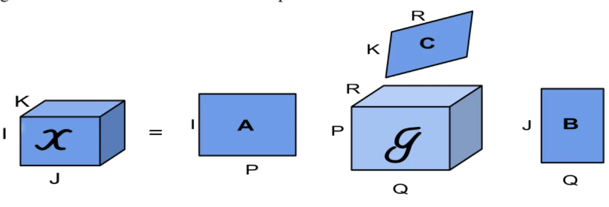
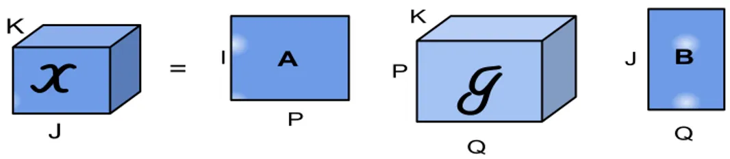
Figure 7 – Illustration of a Tucker decomposition.
=
X
I
J K
B A
P I
G
P
Q R
R
K
J
Q C
Source: Created by the Author
The Tucker decomposition was introduced by Tucker in 1963 [16]. It decomposes the tensor into a core tensor and factor matrices. The PARAFAC decomposition can be viewed as special case of Tucker decomposition, where the core tensorIR is a diagonal tensor. Figure 7
illustrates the Tucker decomposition of a third-order tensorXI×J×K into a core tensorGP×Q×R
and the factor matricesA∈CI×P,B∈CJ×Q andC∈CK×R. The tensorX can be written in n-mode product and scalar forms as
X =G ×1A×2B×3C (2.56)
X(i,j,k)=
P
∑
p=1
Q
∑
q=1
R
∑
r=1
G(p,q,r)A(i,p)B(j,q)C(k,r) (2.57)
2.2.2.1 Uniqueness
In general, the Tucker decomposition is not unique since the core tensor can be transformed by a non-singular matrix and still fit, i.e.
X =G ×1U1×1AU−11×2U2×2BU−21×3U3×3CU−31, (2.58)
=G ×1AU−11U1×2BU2−1U2×3CU−31U3, (2.59)
=G ×1A×2B×3C. (2.60)
In [17], the authors showed that if the core tensor is known, the factor matrices are unique under some scaling factors.
Proof. Consider aN-thorder tensorXI1×···×IN with the core tensorGR1×···×RN and the factor
matricesA(i) of sizeI
matrices. Computing the 1-mode unfolding ofX we have
X(1)=A(1)G(1)(A(N)⊗ ··· ⊗A(2))T (2.61)
Applying Property 2.33 yields
vec(X(1)) = (A(N)
⊗ ··· ⊗A(1))vec(G(1)) (2.62)
ReplacingA(i)byA(i)U(i) we have vec(X(1)) = (A(N)U(N)
⊗ ··· ⊗A(1)U(1))vec(G(1)) = (A(N)
⊗ ··· ⊗A(1))(U(N)⊗ ··· ⊗U(1))(G(1)) (2.63) The equations (2.62) and (2.63) are equal only if the termU(N)
⊗ ··· ⊗U(1)is a identity matrix
meaning thatU(i)=α
iI(i)and N ∏
i=1αi=1, withI
(i) is the identity matrix of sizeR i×Ri.
2.2.2.2 Special Tucker Decompositions
Figure 8 – Illustration of a Tucker-(2,3) decomposition.
=
X
I
J K
B A
P I
G
P
Q K
J
Q
Source: Created by the Author
In [42] the authors introduced the concept of Tucker-(N1,N), whereN denotes the
order of the tensor withN−N1factors matrices equal to the identity matrix. Two decompositions
that are used later in this thesis are the Tucker-(2,3) and Tucker-(1,3).
the decomposition. The tensorX can be expressed as
X =G×1A×2B×3IK (2.64) X(i,j,k)=
P
∑
p=1
Q
∑
q=1
Gp,q,kA(i,p)B(j,q) (2.65)
X..k=AG..kBT (2.66)
whereIK is the identity matrix of sizeK×K andX..k is thek-thfrontal slice ofX. Figure 9 – Illustration of a Tucker-(1,3) decomposition.
=
X
I J K
A
P I
G
P
J K
Source: Created by the Author
The Tucker-(1,3) is the case where the tensor X ∈CI×J×K is decomposed into a core tensorG ∈CP×J×K and a factor matrixA∈CI×P. Figure 9 shows the decomposition. In this case, the tensorX is given by
X =G ×1A×2IJ×3IK (2.67) X(i,j,k)=
P
∑
p=1
A(i,p)G(p,j,k) (2.68)
X..k=AG..k (2.69)
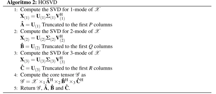
2.2.2.3 Higher-Order Singular Value Decomposition (HOSVD) Algorithm
Tucker decomposition is also known as High-Order Singular Value Decomposition [43]. As explained in the uniqueness section, the Tucker decomposition it’s not unique, meaning that we can only provide a basis for the true factors. In the case, the HOSVD algorithm computes a basis for each factor matrix by via SVD for eachn-mode unfolding of the tensor, selecting
the left singular matrix (if it’s the flatn-mode unfolding) and truncating into the specific size.
Computing the SVD of Equation (2.61) we have
sinceUis an orthogonal matrix that spans the subspace ofA(1)of sizeI
1×R1, and truncatingU
to theR1columns, will exist a non-singular matrixT, of sizeR1×R1, such that
A=UT. (2.71)
However, for a rank-one matrix the uniqueness condition is under some scale factor [44]. The HOSVD algorithm is described in Algorithm 2.
Algoritmo 2:HOSVD
1: Compute the SVD for 1-mode ofX
X(1)=U(1)Σ(1)VH(1)
ˆA=U(1)Truncated to the firstPcolumns 2: Compute the SVD for 2-mode ofX
X(2)=U(2)Σ(2)VH(2)
ˆB=U(2)Truncated to the firstQcolumns 3: Compute the SVD for 3-mode ofX
X(3)=U(3)Σ(3)VH(3)
ˆC=U(3)Truncated to the firstRcolumns 4: Compute the core tensorG as
G =X ×1 ˆAH×2 ˆBH×3 ˆCH 5: ReturnG, ˆA, ˆBand ˆC.
2.2.3 Nested Tucker Decomposition
Figure 10 – 3-D Illustration of aN-thorder Nested Tucker decomposition.
A(1)
C
A(2)C
A(3)C
A(N-1)X
=
(1) (2) (N-2)Source: Created by the Author
Nested Tucker decomposition was introduced in [17]. This decomposition is a general case of the Nested PARAFAC decompositions in [18], where the core tensors are full tensors. This decomposition can be viewed as a special case of the TT decomposition developed by Oseledets in 2011 [35]. The difference is that in the TT decomposition, aN-thorder tensor
is decomposed intoN third-order core tensors with two matrices in the edges, and the Nested
of Tuckers-(1,3) and Tuckers-(2,3)), where those decompositions share a factor matrix. In this thesis, we make use of Nested Tucker decompositions of orders four and five, also referred to as NTD(4) and NTD(5), respectively, to model multi-relaying MIMO systems, as shown in Chapter 4.
Consider theN-thorder tensorXI1×···×IN illustrated in Figure 10, the core tensors
C(n) are of sizeR2n−1×R2n×In+1with exception of the last coreC(N−2)that is of sizeR2n−1× R2n×IN , and the matrices at the edge A(1) andA(N−1) are of size I1×R1 andIN−1×R2N−4,
while the matrices between the coresA(n+1) are of sizeR
2n×R2n+1. This will be clear next
section where the simple cases are introduced. The tensorX can be written as
X(i
1,i2,···,iN)=
R1
∑
r1=1
R2
∑
r2=1
···
RN−1
∑
rN−1=1
A((1i)
1,r1)C (1)
(r1,r2,i2)···C (N−2)
(rN−2,rN−1,iN)A (N−1)
(iN−1,r2N−4) (2.72)
2.2.3.1 Fourth-Order Nested Tucker Decompositions (NTD(4))
Figure 11 – 3-D illustration of a 4-thorder Nested Tucker tensor.
X
=
B
C
U
R
2D
W
I
1R
4I
3R
1I
2R
1R
2R
3R
3I
4R
4Source: Created by the Author
Also called as NTD(4), it decomposes a fourth-order tensor X as a contraction
between a Tucker-(2,3) and Tucker-(1,3) decompositions. The Nested Tucker decomposition of a fourth-order tensorX ∈CI1×I2×I3×I4, illustrated in Figure 11, with factor matrices asB∈CI1×R1,
U∈CR2×R3,D∈CI3×R4 and core tensorsC ∈CR1×R2×I2,W ∈CR3×R4×I4, is written as
X(i
1,i2,i3,i4)=
R1
∑
r1=1
R2
∑
r2=1
R3
∑
r3=1
R4
∑
r4=1
B(i1,r1)C(r
1,r2,i2)U(r2,r3)W(r3,r4,i4)D(i3,r4) (2.73)
Defining the following Tucker-(2,3) and Tucker-(1,3) decompositions:
The tensorX can be viewed as a contraction involvingT (1) andT (2)with the common mode
asR3, i.e. a contraction between a Tucker-(2,3) and Tucker-(1,3) tensors. We have:
X = [(C ×1B×2UT)•12W ]×3D (2.78)
= (C×1B×2UT)•12(W ×2D) (2.79)
=T(1)•12T (2) (2.80)
Alternatively, the tensorX can be viewed as a contraction between tensorsT (3)andT (4)with
the common mode asR2, i.e. a contraction between Tucker-(1,3) and Tucker-(2,3) tensors, i.e.
X = [(C×1B)•12(W ×1U)]×3D (2.81)
= (C×1B)•12(W ×1U×2D) (2.82)
=T (3)•12T (4). (2.83)
In any case, the (i2i4)-thslice ofX is expressed as
X.i2.i4 =BC..i2UW..i4DT∈CI1×I3. (2.84)
2.2.3.2 Fifth-Order Nested Tucker Decomposition (NTD(5))
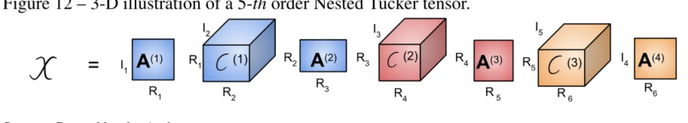
Figure 12 – 3-D illustration of a 5-thorder Nested Tucker tensor.
R2
C
(2) I1R4
R4
R1 I2
R1 R2
R3 R3
I3
R 5
C
(3) R 6I4 R5
I5
R6
C
(1)A
(2)=
X
A
(1)A
(3)A
(4)Source: Created by the Author
This particular case is introduced to simplify the understanding of the MIMO relaying system model in Chapter 4. In this case, we can define the following (2,3) and Tucker-(1,3)
T (1)=C(1)×1A(1)×2A(2)T ∈CI1×R3×I2 (2.85) T (2)=C(2)×2A(3)T ∈CR3×R5×I3 (2.86) T (3)=C(3)×2A(4) ∈CR5×I4×I5 (2.87)
In the NTD(5) case, the tensor X can be viewed as a train of one Tucker-(2,3) and two
Tucker-(1,3) as
and the (.i2i3.i5)-thslice ofX is given by
X.i2i3.i5 =A(1)C (1) ..i2A(2)C
(2) ..i3A(3)C
(3)
..i5A(4)T∈C I1×I4
. (2.89)
2.3 Kronecker Product Approximation
In this section, the Kronecker product approximation is presented. First, we introduce the Van Loan case [32] and then we describe our proposed generalization.
2.3.1 From Kronecker Approximation to Rank-one Matrix
Consider the following Kronecker productX=B⊗C, whereXof sizeRI×SJ,B
of sizeI×JandCof sizeR×Sand the minimization problem
φ(B,C) =||X−B⊗C||F. (2.90) Van Loan in [32] shows that solving (2.90) is the same as solving for a permuted version ofX and then computing a rank-one SVD, as follows
φ(B,C) =||X−vec(B)vec(C)T||F (2.91) A small example can illustrate this rearrangement. Consider asJ=R=S=2 andI=3. The matrixXcan be divided into blocks due to the Kronecker product, as
X=
P(1,1) P(1,2) P(2,1) P(2,2) P(3,1) P(3,2)
, (2.92)
where each blockPis a matrix of size 2×2. The matrixXis constructed as
X=
vec(P(1,1))T vec(P(2,1))T vec(P(3,1))T vec(P(1,2))T vec(P(2,2))T vec(P(3,2))T
(2.93)
Note that this rearrangement maps the elements ofXinto a rank-one matrixXand computing it SVD as
yields a solution forBandCas
ˆB=unvec(√σ1U(:,1)) (2.95) ˆC=unvec(√σ1V∗(:,1)). (2.96)
Note that the estimated ˆBand ˆCare affected by arbitrary scalar factors that compensate each other, i.e.:
B=αˆB (2.97)
C= 1
α ˆC (2.98)
2.3.2 From Kronecker Product Approximation to Rank-one Tensor
In [45], the authors already proposed an extension of the Van Loan’s Kronecker approximation problem to multiple matrices, by rearranging the cost function into tensor product. Consider the generalized minimization problem as
min
A(1)···A(N)||X−A (1)
⊗ ··· ⊗A(N)||F, (2.99)
whereA(i)∈Cpi×qi andX∈CpN···p1×qN···q1. The authors propose to rearrange the cost function
as
||M −S ×3u(3)×4u(4)··· ×N+1u(N+1)||F, (2.100)
whereM ∈CpN×qN×p1q1×···×pN−1qN−1,S =A(N)∈CpN×qN×1andu3···u
N+1are vectors formed
by reshaping the factor matricesA(1)
···A(N−1). Problem (2.100) can be solved by means of the
HOOI (Higher-Order Orthogonal Iterations) algorithm [43].
Our proposed generalization of the Van Loan’s Kronecker approximation consists of rearranging the problem into a rank-one tensor where, comparing to [45], the core tensor is a superdiagonal tensor, i.e. assumes a PARAFAC decomposition. Consider the minimization in (2.99), we proposed a permutation inXsuch that the minimization problem becomes
min
a(1)···a(N)||x−a (1)
⊗ ··· ⊗a(N)||F, (2.101)
wherexis a vectorization of a permuted version ofXand a(i) is the vectorization of theA(i) factor matrix. From Property (2.34), we can rewrite the minimization in (2.102) as
min a(N)···a(1)||
From Definition 8, the tensorX ∈CpNqN×···×p1q1 can be considered as a rank-one tensor. Now,
we consider the special case of a Kronecker product involving the Kronecker product of three matrices: X=A⊗B⊗C. Consider the following cost function:
φ(A,B,C) =||X−A⊗B⊗C||F, (2.103) whereX∈CI1I2I3×R1R2R3,A∈CI3×R3,B∈CI2×R2 andC∈CI1×R1. Minimizing (2.103) is the
same as minimizing the following cost function
φ(a,b,c) =||x−a⊗b⊗c||F ⇐⇒ (2.104) =||X −c◦b◦a||F
wherea=vec(A), b=vec(B),c=vec(C),x=vec(X) is a vector of size I1R1I2R2I3R3×1,
andX is a rank-one tensor of sizeI1R1×I2R2×I3R3.
Due to the Kronecker structure, the matrixXcan be viewed in three different ways: First, as a block matrix of sizeI2I3×R2R3 with each element being a matrix of size I1×R1.
Second, a block matrix of sizeI3×R3, where each element is a matrix of sizeI1I2×R1R2formed
by the blockB⊗C, and, finally, the total matrixX. Our goal is to rearrange the elements ofX into a matrixXsuch thatx=a⊗b⊗c. The matrixXcan be viewed as
X=
[P((11),1)] ··· [P((11),R
2)]
... . .. ...
[P((1I)
2,1)] ··· [P (1) (I2,R2)]
P(2) (1,1)
···
[P((11),1)] ··· [P((11),R
2)]
... . .. ...
[P((1I)
2,1)] ··· [P (1) (I2,R2)]
P(2) (1,R3)
... . .. ...
[P((11),1)] ··· [P((11),R
2)]
... . .. ...
[P((1I)
2,1)] ··· [P (1) (I2,R2)]
P((2I)
3,1)
···
[P((11),1)] ··· [P((11),R
2)]
... . .. ...
[P((1I)
2,1)] ··· [P (1) (I2,R2)]
P((2I)
3,R3)
P(3) (1,1)
(2.105)
where each blockP(1) is a matrix of sizeI
1×R1, each blockP(2)is a matrix of sizeI1I2×R1R2,
and the blockP(3)is the total matrix of sizeI
1I2I3×R1R2R3. The sub indices only indicates the
block position in reference to the big block, e.g. the sub indices of P((11),1) indicates that is the first block in the bigger block P((2n),m), wheren={1···I3}andm={1···R3}. After this block
of each blockP(1) in the bigger blockP(2)
(n,m), following the row sense. X(n,m)= [vec(P((11),1)); vec(P((1I)
2,1));···; vec(P (1)
(I2,R2))]P((2n),m).
Defining the matrixXof sizeI1R1I2R2×I3R3as the matrix whose column vectors are formed
by vec(X(n,m))
X= [vec(X(1,1));···; vec(X(I3,1));
···; vec(X(I3,R3))] (2.106)
Equation (2.106) represents our rearrangement, i.e. vec(X) =a⊗b⊗c, andX is the third-order
rank-one tensor of sizeI1R1×I2R2×I3R3, given by the tensorization ofx. This tensor can be
written as
X =c◦b◦a. (2.107)
In this case, we approximate a matrix by the Kronecker product of three matrices by rearranging it as a third-order rank-one tensor, the matrices can be estimated, for example, by using the ALS algorithm or the HOSVD algorithm and it will be unique with some scaling factor.
Next, a simple example of the rank-one tensor approximation of the Kronecker product of three matrices,X=A⊗B⊗C, with the matrices defined as
A=
a1 a3
a2 a4
B=
b1 b3
b2 b4
C=
c1 c3
c2 c4
. (2.108)
Also, we have the vectorsa=vec(A),b=vec(B)andc=vec(C),
a= a1 a2 a3 a4 b= b1 b2 b3 b4 c= c1 c2 c3 c4 . (2.109)
Definingx=a⊗b⊗c, we have:
x=
a1b1c1
a1b1c2
a1b1c3
...
a4b4c4
64×1
(2.110)