DEPARTAMENTO DE ENGENHARIA DE TELEINFORM ´ATICA
PROGRAMA DE P ´OS-GRADUAC¸ ˜AO EM ENGENHARIA DE TELEINFORM ´ATICA
PAULO RICARDO BARBOZA GOMES
TENSOR METHODS FOR ARRAY PROCESSING AND CHANNEL ESTIMATION IN WIRELESS COMMUNICATIONS SYSTEMS
FORTALEZA
Tese apresentada ao Programa de P´os-gradua¸c˜ao em Engenharia de Teleinform´atica do Departamento de Engenharia de Telein-form´atica da Universidade Federal do Cear´a, como parte dos requisitos necess´arios para a obten¸c˜ao do t´ıtulo de Doutor em Engenharia de Teleinform´atica. ´Area de concentra¸c˜ao: Sinais e Sistemas. Linha de pesquisa: Pro-cessamento de Sinais e Imagens.
Orientador: Prof. Dr. Andr´e Lima F´errer de Almeida (UFC)
Coorientador: Prof. Dr. Jo˜ao Paulo Car-valho Lustosa da Costa (UnB)
Gerada automaticamente pelo módulo Catalog, mediante os dados fornecidos pelo(a) autor(a)
G616t Gomes, Paulo Ricardo Barboza.
Tensor methods for array processing and channel estimation in wireless communications systems / Paulo Ricardo Barboza Gomes. – 2018.
136 f. : il. color.
Tese (doutorado) – Universidade Federal do Ceará, Centro de Tecnologia, Programa de Pós-Graduação em Engenharia de Teleinformática, Fortaleza, 2018.
Orientação: Prof. Dr. André Lima Férrer de Almeida.
Coorientação: Prof. Dr. João Paulo Carvalho Lustosa da Costa.
1. Tensor Modeling. 2. Array Processing. 3. Wireless Communications Systems. 4. Parameters Estimation. 5. Channel Estimation. I. Título.
do Departamento de Engenharia de Telein-form´atica da Universidade Federal do Cear´a, como parte dos requisitos necess´arios para a obten¸c˜ao do t´ıtulo de Doutor em Engenharia de Teleinform´atica. Area de concentra¸c˜ao:´ Sinais e Sistemas. Linha de pesquisa: Pro-cessamento de Sinais e Imagens.
Aprovada em: 21 / 09 / 2018.
BANCA EXAMINADORA
Prof. Dr. Andr´e Lima F´errer de Almeida (Orientador) Universidade Federal do Cear´a (UFC)
Prof. Dr. Jo˜ao Paulo Carvalho Lustosa da Costa (Coorientador) Universidade de Bras´ılia (UnB)
Prof. Dr. Jo˜ao Cesar Moura Mota Universidade Federal do Cear´a (UFC)
Prof. Dr. Walter da Cruz Freitas J´unior Universidade Federal do Cear´a (UFC)
Prof. Dr. Marcello Luiz Rodrigues de Campos Universidade Federal do Rio de Janeiro (UFRJ)
Prof. Dr. G´erard Favier
entender durante esse longo tempo todas as ren´uncias com paciˆencia, motiva¸c˜ao e carinho. Serei eternamente grato. Amo vocˆes!
Ao meu orientador Prof. Dr. Andr´e Lima F´errer de Almeida, e ao meu coorientador Prof. Dr. Jo˜ao Paulo Carvalho Lustosa da Costa, pela excelente orienta¸c˜ao, li¸c˜oes, paciˆencia, disponibilidade, oportunidades e amizade durante esses longos anos. A humildade e entusiasmo de vocˆes me inspiram a ser um profissional de excelˆencia. Muito obrigado por me guiarem nesta conquista!
`
A toda a equipe do Grupo de Pesquisa em Telecomunica¸c˜oes sem Fio (GTEL), especialmente aos professores Dr. Francisco Rodrigo Porto Cavalcanti, Dr. Jo˜ao Cesar Moura Mota e Dr. Tarcisio Ferreira Maciel, pelos ensinamentos e oportunidades profis-sionais a mim concedidas.
`
A todos os amigos, especialmente, Fernando Filho, Joyce, R´egis Wendel, Vl´adia, Lucas, Karine, Bernardinho, Bruno R´egis, R´egis Lima, Ana Vanessa, Ana Lara e Albano. Vocˆes s˜ao uma extens˜ao da minha fam´ılia!
`
A UFC, GTEL, FUNCAP, Ericsson Telecomunica¸c˜oes S/A e LG Eletronics do Brasil, pela estrutura e suporte financeiro durante o per´ıodo de doutorado.
`
A todas as pessoas que, de alguma maneira, contribu´ıram direta ou indireta-mente para a realiza¸c˜ao deste trabalho. Os meus sinceros agradecimentos!
Senhor, fazei de mim um instrumento da vossa paz.
Onde h´a ´odio, que eu leve o amor. Onde h´a ofensa, que eu leve o perd˜ao. Onde h´a disc´ordia, que eu leve a uni˜ao. Onde h´a d´uvida, que eu leve a f´e. Onde h´a erro, que eu leve a verdade.
Onde h´a desespero, que eu leve a esperan¸ca. Onde h´a tristeza, que eu leve a alegria. Onde h´a trevas, que eu leve a luz.
´
O Mestre,
Fazei que eu procure mais consolar que ser consolado
compreender que ser compreendido; amar que ser amado.
Pois ´e dando que se recebe, ´e perdoando que se ´e perdoado,
´e morrendo que se vive para a vida eterna.
desses sistemas devido `a estimativas de parˆametros mais acuradas (por exemplo: dire¸c˜ao de partida, dire¸c˜ao de chegada, atraso, frequˆencia Doppler, coeficientes de canal, ru´ıdo de fase) apresentando melhores condi¸c˜oes de identificabilidade. Nesse contexto, esta tese prop˜oe novas modelagens tensoriais para processamento de sinais em arranjos e estima¸c˜ao de canal aplicada `a sistemas de comunica¸c˜oes sem-fio. Na primeira parte desta tese, dedicada `a processamento de sinais em arranjos multidimensionais de sensores e radar, propomos uma nova t´ecnica de pr´e-processamento tensorial para supress˜ao de ru´ıdo que reduz significantemente o efeito do ru´ıdo em dados matriciais e tensoriais implicando em melhores estimativas dos parˆametros desejados. Em seguida, novas modelagens tensoriais baseadas nas decomposi¸c˜oes PARAFAC, Tucker e Nested-PARAFAC s˜ao formuladas, a partir das quais novos algoritmos para estima¸c˜ao conjunta de ˆangulo de partida e ˆangulo de chegada s˜ao propostos. Na segunda parte deste documento, modelagens tensoriais s˜ao desenvolvidas para resolver o problema de estima¸c˜ao de canal em sistemas de comu-nica¸c˜oes MIMO sem-fio. Primeiramente, propomos um esquema de codifica¸c˜ao e retrans-miss˜ao multi-frequencial que concentra o processamento associado `a estima¸c˜ao conjunta dos canais de downlink e uplink na esta¸c˜ao-base. Mostramos que o sinal retransmitido recebido pode ser modelado como a decomposi¸c˜ao PARAFAC de um tensor de terceira-ordem. Em seguida, a decomposi¸c˜ao PARAFAC ´e novamente explorada na modelagem de um sistema de comunica¸c˜ao MIMO mais realista que considera perturba¸c˜oes de ru´ıdos de fase em cada antena transmissora e receptora. Algoritmos receptores para estima¸c˜ao de canal e ru´ıdo de fase s˜ao formulados. Resultados de simula¸c˜ao s˜ao apresentados para ilustrar o desempenho dos receptores propostos que s˜ao comparados ao estado-da-arte.
In several applications in the field of digital signal processing, for example, wireless com-munications, sonar and radar, the received signal has a multidimensional nature which can intrinsically include on its structure many dimensions such as space, time, frequency, code, and polarization. In view of this, modern processing techniques which exploit all the signal dimensions can be developed to improve the system performance due to more accurate parameter estimation (for example: direction of departure, direction of arrival, delay, Doppler frequency, channel coefficients, phase noise) with powerful identifiability conditions. In this context, this thesis proposes new tensor modeling approaches for ar-ray processing and channel estimation applied to wireless communications systems. In the first part of this thesis, devoted to multidimensional sensor array and radar process-ing, we propose a new tensor-based preprocessing technique for noise supression which significantly reduces the noise effect in matrix and tensor data leading to more accu-rate estimates of the desired parameters. Then, new tensor methods capitalizing on the PARAFAC, Tucker and Nested-PARAFAC decompositions are formulated, from which new algorithms for joint direction of departure and direction of arrival estimation are pro-posed. In the second part of this document, tensor modeling approaches are developed to solve channel estimation problems in MIMO wireless communications systems. Firstly, we propose a new closed-loop and multi-frequency channel training framework that con-centrates the processing associated with joint downlink and uplink channel estimation at the base station. We also show that the received closed-loop signal can be modeled as the PARAFAC decomposition of a third-order tensor. Then, the PARAFAC decomposition is also exploited to modeling a more realistic MIMO communication system that considers phase noise perturbations at each transmit and receive antenna. Receiver algorithms for channel and phase noise estimation are formulated. Simulation results are presented to il-lustrate the performance of the proposed receivers which are compared to state-of-the-art approaches.
Figure 4 – Construction process of the 1-mode, 2-mode and 3-mode unfolding ma-trices of a third-order tensor from its frontal, horizontal and lateral slices. Source: Adapted from (Ximenes, 2015) . . . 35 Figure 5 – PARAFAC decomposition of X ∈CI1×I2×I3 intoQ components. Source:
Adapted from (de Almeida, 2007) . . . 37 Figure 6 – Tucker decomposition of a third-order tensor X ∈ CI1×I2×I3. Source:
Adapted from (de Almeida, 2007) . . . 42 Figure 7 – Illustration of spatial smoothing and sensors in common for lr = 2
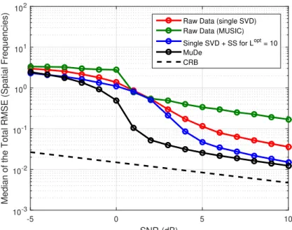
sub-arrays in the r-th spatial dimension. Source: Created by the author. . . . 51 Figure 8 – SNRoutput vs. SNRinput for a third-order tensor to compare the SNR gain
of MuDe and the classical single HOSVD based low-rank approximation proposed by (Haardt, Roemer, and del Galdo, 2008). In the simulated scenario: URA, N1 = 30, N2 = 30, M = 6 and K = 10. Source: Created
by the author. . . 54 Figure 9 – Median of the total RMSE of the spatial frequencies vs. SNR (dB) for a
third-order tensor to compare the spatial parameter estimation accuracy. In the scenario: URA, N1 = 30, N2 = 30, M = 6 and K = 10. Source:
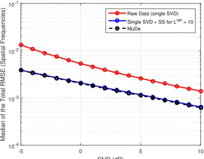
Created by the author. . . 54 Figure 10 –Median of the total RMSE of the spatial frequencies vs. SNR (dB) for
the matrix-based approach. In the scenario: ULA, N = 30, M = 6 and
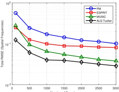
K = 30. Source: Created by the author. . . 55 Figure 11 –Median of the total RMSE of the spatial frequencies vs. SNR (dB) for
the matrix-based approach. In the scenario: ULA, N = 30, M = 1 and
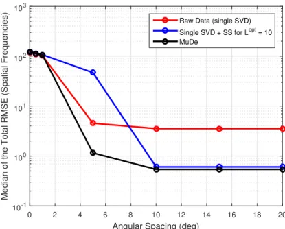
K = 30. Source: Created by the author. . . 56 Figure 12 –Median of the total RMSE of the spatial frequencies vs. angular spacing
(in degrees) between the sources. In the scenario: ULA, N = 30, M = 5,
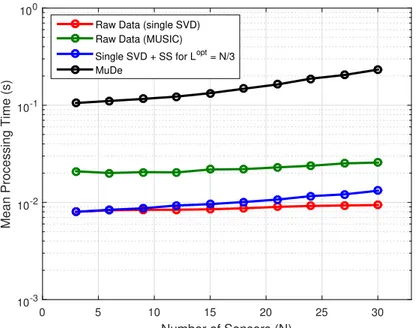
K = 30 and SNR equal to 0 dB. Source: Created by the author. . . 57 Figure 13 –Mean processing time (in seconds) vs. number of sensors. In the
Figure 14 –L-shaped array configuration with N1 +N2 −1 sensors. The distance
between the sensors in the z axis is d(1) while the distance between the
sensors in the x axis is d(2). The m-th wavefront has elevation and
az-imuth angles equal to αm and βm, respectively. Source: Created by the author. . . 64 Figure 15 –Total RMSE vs. SNR for N = 64 sensors, K = 10 samples, DoAs:
{30◦,55◦} and {45◦,60◦} for Hadamard sources’ sequences. Uniform
re-tangular array (URA). Source: Created by the author. . . 68 Figure 16 –Total RMSE vs. SNR for N = 64 sensors, K = 10 samples, DoAs:
{30◦,55◦
} and {45◦,60◦
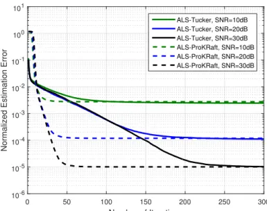
} for BPSK sources’ sequences. Uniform retan-gular array (URA). Source: Created by the author. . . 68 Figure 17 –Convergence of the iterative ALS-Tucker and ALS-ProKRaft algorithms.
Uniform retangular array (URA). Source: Created by the author. . . 69 Figure 18 –Total RMSE vs. SNR for N = 13 sensors, K = 500 samples, DoAs:
{30◦,45◦
} and {50◦,55◦
}. L-Shaped array. Source: Created by the author. 70 Figure 19 –Total RMSE vs. SNR (performance of the ALS-Tucker algorithm for
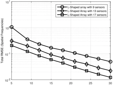
different number os sensors). L-Shaped array. Source: Created by the author. . . 70 Figure 20 –Total RMSE vs. number of samples. L-Shaped array. Source: Created
by the author. . . 71 Figure 21 –Bistatic MIMO radar scenario. Source: Adapted from (Wanget al., 2018) 75 Figure 22 –Total RMSE (deg) vs. positioning error factor (α). Source: Created by
the author. . . 84 Figure 23 –Number of iterations for convergence vs. SNR (dB). Source: Created by
the author. . . 84 Figure 24 –Mean processing time (in seconds) vs. data block size. Source: Created
by the author. . . 85 Figure 25 –Conventional training framework. The DL and UL channel estimation problems
are solved independently. The BS first transmits pilot signals. Then, the DL channel is estimated at the MSs side. The estimated DL channel is feed back to the BS via dedicated uplink resources. The UL channel is estimated at the BS side. The blue words refer to DL communication, while red words refer to UL communication. Source: Created by the author. . . . 91 Figure 26 –Proposed closed-loop and multi-frequency based training framework. The
the author. . . . 98 Figure 29 –NMSE (DL and UL Channels) vs. number of subcarriers (F) for N = 32,
T = 16,U = 4 and SNR = 10 dB.Source: Created by the author. . . . 99 Figure 30 –NMSE (DL and UL Channels) vs. length of the training sequence (T) for
N = 32,F = 4,U = 4 and SNR = 10 dB.Source: Created by the author. . . . 100 Figure 31 –Number of iterations for convergence of the proposed ALS-PARAFAC receiver
vs. SNR (dB) for N = 32, T = 16 andU = 4. Source: Created by the author. . 100 Figure 32 –NMSE vs. number of transmission beams (P) for the DL channel
esti-mation, U = 2, T = 16 and F = 25. Source: Created by the author. . . . 107 Figure 33 –NMSE vs. number of reception beams (Q) for the UL channel estimation,
U = 2, T = 16 and F = 25. Source: Created by the author. . . 107 Figure 34 –NMSE vs. number of subcarriers (F) for the DL channel estimation,
U = 2 and T = 16. Source: Created by the author. . . 108 Figure 35 –NMSE vs. number of subcarriers (F) for the UL channel estimation,
U = 2 and T = 16. Source: Created by the author. . . 108 Figure 36 –NMSE vs. length of the pilot signal (T) for the DL channel estimation,
U = 2, P = 8 andF = 25. Source: Created by the author.. . . 109 Figure 37 –NMSE vs. length of the pilot signal (T) for the UL channel estimation,
U = 2, P = 8 andF = 25. Source: Created by the author.. . . 109 Figure 38 –Frequency-selective MIMO system equipped with different oscilators at
the M transmit andN receive antennas. Source: Adapted from (Huang, Wang, and He, 2015). . . 113 Figure 39 –Illustration of frame and sub-frame structures. The pilot symbols part
SP is reused frame to frame. The PN is invariant within a sub-frame while the channel gains remain constant over the length of one frame1. Source: Created by the author. . . . 113
Figure 40 –NMSE of ˆH vs. SNR (dB) of a 4×4 MIMO system for different pilot length (LP), LD = 100 and BPSK modulation. Source: Created by the author. . . 120 Figure 41 –NMSE of ˆΦ[t] vs. SNR (dB) of a 4×4 MIMO system for different pilot
Figure 42 –NMSE of ˆΦ[r] vs. SNR (dB) of a 4×4 MIMO system for different pilot length (LP), LD = 100 and BPSK modulation. Source: Created by the author. . . 121 Figure 43 –BER vs. SNR (dB) of a 4×4 MIMO system with perfect and imperfect
channel and PN knowledge for different pilot length (LP),LD = 100 and BPSK modulation. Source: Created by the author. . . 122 Figure 44 –Number of iterations for convergence vs. SNR (dB) of a 4×4 MIMO
ALS Alternating Least Squares AoA Angle of Arrival
AoD Angle of Departure
AWGN Additive White Gaussian Noise BALS Bilinear Alternating Least Squares BER Bit Error Rate
BPSK Binary Phase Shift Keying
BS Base Station
CANDECOMP CANonical DECOMPosition
CP CANDECOMP/PARAFAC
CRB Cramer-Rao Bound CS Compressed Sensing
CSI Channel State Information
DALS Double Alternating Least Squares
dB Decibel
DFT Discrete Fourier Transform
DL Downlink
DoA Direction of Arrival DoD Direction of Departure
DS-CDMA Direct-Sequence Code-Division Multiple Access
ESPRIT Estimation of Signal Parameters via Rotational Invariance Technique FBA Forward-Backward Averaging
FDD Frequency Division Duplexing
FISTA Fast Iterative Shrinkage-Thresholding FLOP Floating Point Operation
FR Frequency Range
GNSS Global Navigation Satellite System HB Hybrid Analog-Digital Beamforming
HOSVD Higher Order Singular Value Decomposition
i.i.d. Independent and Identically Distributed Random Variables
LS Least-Squares
LS-KRF Least-Squares Khatri-Rao Factorization MIMO Multiple-Input Multiple-Output
MMSE Minimum Mean Square Error mmWave Millimeter Wave
NR New Radio
NULA Non-Uniform Linear Array
OFDM Orthogonal Frequency Division Multiplexing OMP Orthogonal Matching Pursuit
OPA Outer Product based Array OPP Orthogonal Procrustes Problem PARAFAC PARAlell FACtor
PM Propagator Method
PN Phase Noise
ProKRaft Procrustes Estimation and Khatri-Rao Factorization
R-D Multidimensional Sensor Array RF Radio Frequency
RMSE Root Mean Square Error
S-CosaMP Structured Compressive Sampling Matching Pursuit SISO Single-Input Single-Output
SNR Signal-to-Noise Ratio SS Spatial Smoothing STF Space-Time-Frequency
SVD Singular Value Decomposition TALS Trilinear Alternating Least Squares TDD Time Division Duplexing
UL Uplink
Throughout this thesis the following conventions are used. Scalars are de-noted by lower-case lettersx, column vectors as boldface lower-case lettersx, matrices as boldface upper-case lettersX, and tensors as boldface calligraphic letters X.
C set of complex-valued numbers
CI set of complex-valued I-dimensional vectors CI×Q set of complex-valued (I ×Q)-matrices
CI1×I2×···×IN set of complex-valued (I
1×I2× · · · ×IN)-tensors
{·}∗ complex conjugate
{·}T transpose
{·}H conjugate transpose
{·}−1 inverse
{·}† Moore-Penrose pseudo-inverse
k · kF Frobenius norm
⊗ Kronecker product
⋄ Khatri-Rao (column-wise Kronecker) product
◦ outer product
xi,q (i, q)-th element of X ∈CI×Q
xi1,i2,···,iN (i1, i2,· · · , iN)-th element of X ∈C
I1×I2×···×IN
xq q-th column ofX ∈CI×Q X(i,:) i-th row of X ∈CI×Q
X(i:k,:), i < k submatrix fomed by the i-th toj-th row of X
Xi1·· i1-th horizontal slice of X ∈CI1×I2×I3
X·i2· i2-th lateral slice of X ∈C
I1×I2×I3
X··i3 i3-th frontal slice of X ∈CI1×I2×I3
[X](n) n-mode unfolding matrix of X ∈CI1×I2×···×IN
×n n-mode product
IN identity matrix of size N ×N
IN,Q identity tensor of N-th order and rank-Q
ρx rank of X
κx Kruskal-rank (k-rank) of X
E{·} expectation operator
⊔n concatenation operator along n-th mode of X vec (·) vectorization operator
unvec (·) unvectorization operator (inverse of the vectorization operator) vecd (·) converts the main diagonal of a matrix into a column vector
1 INTRODUCTION . . . 22
1.1 Thesis Scope and Motivation . . . 22
1.2 Main Contributions . . . 24
1.3 Thesis Organization . . . 24
1.4 Scientific Production . . . 26
1.4.1 Participation in Research Projects . . . 26
1.4.2 Journal Papers . . . 27
1.4.3 Conference Papers . . . 27
1.4.4 Patent . . . 28
2 PREREQUISITES OF MULTILINEAR ALGEBRA . . . 29
2.1 Matrix Products and Operators . . . 29
2.2 Matrix Factorizations . . . 30
2.2.1 Singular Value Decomposition (SVD) . . . 30
2.2.2 Least-Squares Khatri-Rao Factorization (LS-KRF) . . . 31
2.3 Tensor Definitions and Operations . . . 33
2.4 Tensor Decompositions . . . 36
2.4.1 PARAFAC Decomposition . . . 36
2.4.2 Nested-PARAFAC Decomposition . . . 40
2.4.3 Tucker Decomposition . . . 42
2.5 Chapter Summary . . . 45
3 TENSOR-BASED METHODS FOR BLIND SPATIAL SIG-NATURE ESTIMATION IN MULTIDIMENSIONAL SENSOR ARRAYS . . . 46
3.1 Introduction and Motivation . . . 46
3.1.1 Chapter Organization . . . 48
3.2 Data Model . . . 48
3.6 Proposed Tensor-Based Methods for Blind Spatial Signature
Estimation . . . 59
3.6.1 Covariance Tensor Formulation . . . 59
3.6.2 ALS-Tucker Algorithm . . . 60
3.6.3 ALS-ProKRaft Algorithm . . . 61
3.7 Spatial Signature Estimation in L-Shaped Sensor Arrays . . . . 63
3.7.1 Cross-Correlation Tensor for L-shaped Sensor Arrays . . . 64
3.7.2 Estimation of the Spatial Frequencies . . . 66
3.8 Computational Complexity . . . 66
3.9 Advantages and Disadvantages of the Proposed Methods . . . 66
3.10 Performance Evaluation of ALS-Tucker and ALS-ProKraft Al-gorithms . . . 67
3.11 Chapter Summary . . . 71
4 A NESTED-PARAFAC BASED APPROACH FOR TARGET LOCALIZATION IN BISTATIC MIMO RADAR SYSTEMS . 73 4.1 Introduction and Motivation . . . 73
4.1.1 Chapter Organization . . . 74
4.2 Signal Model . . . 75
4.3 Proposed Tensor-Based Method for Joint DoD and DoA Esti-mation . . . 76
4.3.1 Proposed Nested-PARAFAC Based Modeling . . . 78
4.3.2 First ALS Stage (Trilinear ALS) . . . 79
4.4 Uniqueness Issues . . . 82
4.5 Computational Complexity . . . 83
4.6 Simulation Results . . . 83
4.7 Chapter Summary . . . 86
5 JOINT DOWNLINK AND UPLINK CHANNEL ESTIMA-TION USING TENSOR PROCESSING . . . 87
5.1 Introduction and Motivation . . . 87
5.1.1 Chapter Organization . . . 89
5.2 System Model . . . 89
5.2.1 Downlink Signal Model . . . 89
5.2.2 Uplink Signal Model . . . 89
5.2.3 Conventional x Proposed Channel Training Framework . . . 90
5.3 Proposed Tensor-Based Semi-Blind Receivers for Joint DL and UL Channel Estimation . . . 92
5.3.1 PARAFAC-Based Modeling . . . 92
5.3.2 ALS-PARAFAC Receiver . . . 93
5.3.3 LS-KRF Receiver . . . 94
5.4 Identifiability and Computational Complexity . . . 95
5.4.1 Identifiability Conditions . . . 96
5.4.2 Computational complexity . . . 97
5.5 Simulation Results (Part 1) . . . 97
5.6 Extension to mmWave Massive MIMO Systems . . . 101
5.6.1 Sparse Formulation for DL and UL Channel Parameters Esti-mation . . . 104
5.6.2 Identifiability Condition . . . 106
5.7 Simulation Results (Part 2) . . . 106
6.3 Proposed PARAFAC-Based Modeling . . . 114 6.4 Proposed Semi-Blind Receiver for Joint Channel and PN
1 INTRODUCTION
This is an introductory chapter where we present the motivation and scope of this thesis in Section 1.1. After that, we present our main contributions in Section 1.2, followed by the thesis overview in Section 1.3. Finally, the main scientific production produced during the doctoral period are presented in Section 1.4.
1.1 Thesis Scope and Motivation
High resolution parameter estimation and channel estimation problems play fundamental roles in several practical applications in the field of digital signal processing. For example, the first one ranging from array processing in radar, sonar, acoustics and global navigation satellite systems (GNSS), to name a few, while the latter is commonly applied to mobile communications systems. Conventional signal processing techniques usually consider only the space and time dimensions which leads to matrix-based model-ing. However, often the space domain can be split into two signal dimensions (azimuth and elevation), while the time domain can be divided into other two dimensions (frames and sub-frames) so that the received signal to be processed has a multidimensional nature which can also include on its structure other dimensions (for example: frequency, code and polarization) that are not take into account since matrices are only two-dimensional data structures. In view of this, modern processing techniques that extend the existing approaches by exploiting all the signal dimensions can be developed by using tensor tools. There are significant advantages of using tensor-based signal processing instead of matrix-based signal processing. Among these advantages, we can cite the improved identifiability conditions, which generally come from the essential uniqueness property of tensor decom-positions. Tensor-based methods also inherits the so-calledtensor gain, which translates into improved accuracy due to the efficient noise rejection capability (da Costa et al., 2011; Roemer, 2013).
In the context of wireless communications systems, the authors of the seminal work (Sidiropoulos, Giannakis, and Bro, 2000) proposed a blind multiuser separation for direct-sequence code-division multiple access (DS-CDMA) by modeling the received signal as a third-order PARAFAC decomposition. de Almeida, Favier, and Mota (2007) proposes a unified PARAFAC-based modeling with application to blind multiuser equalization. In works (Liu et al., 2013) and (de Almeida et al., 2013), different tensor-based receivers are formulated to solving the joint symbol and channel estimation problem in space-time-frequency (STF) MIMO communication systems. In the former, the PARAFAC decomposition is exploited to derive a closed-form solution based on the factorization of the Khatri-Rao product. The latter proposed a blind receiver that exploits a general-ized PARATUCK2 model (Harshman and Lundy, 1996) of the STF-MIMO transmission system.
Nowadays, millimeter wave (mmWave) MIMO communication systems has been subject of increasing interest in both academia and industry since it is a promising technology for future 5G mobile communication systems due to its potential to offer gigabit-per-second data rates by exploiting the large bandwidth available at mmWave frequencies (Zhou et al., 2016a). This has motived the development of new tensor-based approaches for mmWave MIMO channel estimation. In this way, the authors of (Zhou et al., 2016a) proposed a layered pilot transmission scheme and explored the intrinsic low-rank structure of the received signal, resulting of the sparse scattering nature of the mmWave channel, to formulate a PARAFAC-based method for the joint estimation of the uplink channels of multiple users assuming channel reciprocity. In (Zhou et al., 2017), the same authors studied the downlink channel estimation problem for frequency-selective mmWave MIMO channels. Similarly, the received signal is organized into a third-order tensor which admits a PARAFAC decomposition and the channel parameters (angles of departure and arrival, time delays and fading coefficients) are jointly estimated from the decomposed factor matrices. In contrast to (Zhou et al., 2017), the authors of (Ara´ujo and de Almeida, 2017) explore both the sparse and multidimensional structures of frequency-selective mmWave MIMO channels and recast the channel estimation problem as a multi-way compressed sensing problem. The channel parameters are estimated by solving a simpler compressive sensing problem for each channel dimension.
2009). Additionally, one can also benefit from the multidimensional structure of tensor data to perform noise rejection/prewhitening, as shown in (da Costa et al., 2011).
1.2 Main Contributions
In this thesis, we propose new tensor-based modeling and algorithms to solve parameter estimation problems in array processing, as well as channel and phase noise estimation problems in MIMO wireless communications systems. The main contributions can be summarized as follows:
• Development of a new denoising framework for matrix and tensor data to improve the parameter estimation accuracy in multidimensional sensor array processing;
• New tensor-based formulations for the covariance structure of the received signal in multidimensional sensor arrays and bistatic MIMO radar systems exploiting the PARAFAC, Nested-PARAFAC and Tucker decompositions;
• Development of new PARAFAC, Nested-PARAFAC and Tucker-based receiver al-gorithms for direction of departure and direction of arrival estimation in multidi-mensional sensor arrays and bistatic MIMO radar systems;
• Proposal of a new PARAFAC-based channel training framework and development of receiver algorithms which concentrate the joint downlink and uplink channel estimation at the BS side in MIMO wireless communications systems ;
• Development of a new PARAFAC-based approach for the joint channel and phase noise estimation in MIMO communication systems;
• Study of the identifiability issues and computational complexities of the proposed methods.
1.3 Thesis Organization
This thesis is divided into seven chapters, including this introductory chapter. In the following, we briefly describe the content of the six remaining chapters.
Chapter 2: Prerequisites of Multilinear Algebra. This chapter provides a theoretical basis for the methods developed in this thesis. It first review important definitions and operations of multilinear algebra. Then, the three most important tensor decompositions to the context of this thesis, namely PARAFAC, Nested-PARAFAC and Tucker decompo-sitions are introduced. The contribution presented in this chapter is to unify in one place fundamental concepts spread in the literature in order to make it easily understandable for the reader.
sor and matrix data. In the second part, the covariance matrix of the received signal is formulated as a PARAFAC model (for uncorrelated sources) and as a Tucker model (for correlated sources). Two generalized iterative algorithms for direction of arrival estima-tion are proposed.
Chapter 4: A Nested-PARAFAC Approach for Target Localization in Bistatic MIMO Radar Systems. This chapter addresses the target localization problem in bistatic MIMO radar systems. We formulate a new tensor modeling for the cross-covariance matrix of the matched filters outputs using a Nested-PARAFAC decomposition, from which two receiver algorithms are proposed to jointly estimate the directions of departure and arrival of multiple targets located at the same range bin of interest. Identifiability issues and computational complexity of the proposed algorithms are also discussed.
The second part of this thesis, which comprises Chapters 5 and 6, is devoted to solve the problem of channel and phase noise estimation in MIMO wireless communi-cations systems.
Chapter 5: Joint Downlink and Uplink Channel Estimation Using Tensor Processing. This chapter addresses the problem of channel estimation in MIMO wireless communica-tions systems. Initially, a novel closed-loop and multi-frequency based channel training framework is presented. It allows to concentrate most of the processing burden for channel estimation at the base station, i.e., avoiding such processing at the mobile stations side. We formulate a new PARAFAC-based modeling for the received closed-loop signal. We also extend the proposed tensor signal model for millimeter-wave MIMO scenarios. Two new semi-blind receivers to perform the joint downlink and uplink channel estimation are developed, and identifiability issues and computational complexity are studied.
Chapter 7: This chapter concludes the thesis by summarizing the obtained results and listing some perspectives for future work.
Remark: This thesis has four chapters with the main contributions that cover different aspects of array signal processing and channel estimation in MIMO wireless communications systems. Every chapter is meant to be self-contained so that the reader can read them independently without loss of information.
1.4 Scientific Production
The experiences in research projects as well as the technical reports and pub-lications produced during the doctoral period are listed as follows.
1.4.1 Participation in Research Projects
• Speech Processing for Far Field Automatic Speech Recognition. March/2015 - Febru-ary/2016. Developed under the context of LG Electronics/UFC technical coopera-tion projects;
• UFC.44 Hybrid Beamforming and Massive MIMO for 5G Wireless Systems. Octo-ber/2016 - September 2018. Developed under the context of Ericsson/UFC technical cooperation projects,
in which a number of four technical reports in UFC.44 were delivered:
• Paulo R. B. Gomes, and Andr´e L. F. de Almeida, Joint DL and UL Chan-nel Estimation Using Tensor Processing. First Technical Report (TR01) UFC.44. GTEL-UFC, April, 2017;
• Paulo R. B. Gomes, and Andr´e L. F. de Almeida,Joint DL and UL Channel Es-timation for Massive MIMO Communications Using Hybrid Beamforming. Second Technical Report (TR02) UFC.44. GTEL-UFC, October, 2017;
• Paulo R. B. Gomes, and Andr´e L. F. de Almeida,Multidimensional User Group-ing for Frequency-Selective MU-MIMO Systems. Third Technical Report (TR03) UFC.44. GTEL-UFC, April, 2018.
• Paulo R. B. Gomes, Francisco H. C. Neto, Weskley V. F. Maur´ıcio, Daniel C. Ara´ujo, Andr´e L. F. de Almeida, and Tarcisio F. Maciel, Hybrid Beamforming De-sign Exploiting Implicit and Explicit CSI in Massive MIMO Systems. Fourth Tech-nical Report (TR04) UFC.44. GTEL-UFC, September, 2018.
vol. 62, pp. 197-210, 2017;
• Paulo R. B. Gomes, Andr´e L. F. de Almeida, Jo˜ao Paulo C. L. da Costa, Jo˜ao C. M. Mota, Daniel Valle de Lima, and G. Del Galdo, Tensor-Based Methods for Blind Spatial Signature Estimation in Multidimensional Sensor Arrays, in International Journal of Antennas and Propagation, vol. 2017, pp. 1-11, 2017;
• Paulo R. B. Gomes, Jo˜ao Paulo C. L. da Costa, and Andr´e L. F. de Almeida, Tensor-Based Multiple Denoising via Successive Spatial Smoothing, Low-Rank Ap-proximation and Reconstruction for R-D Sensor Array Processing, in Digital Signal Processing, May 2018. Under Major Revision;
• Paulo R. B. Gomes, Andr´e L. F. de Almeida, and Jo˜ao Paulo C. L. da Costa, A Nested-PARAFAC Based Approach for Target Localization in Bistatic MIMO Radar Systems, in Digital Signal Processing, April, 2018. Under Review;
• Paulo R. B. Gomes, Andr´e L. F. de Almeida, Jo˜ao Paulo C. L. da Costa, and Rafael T. de Sousa Jr., Tensor-Based Semi-Blind Receiver for Joint Channel and Phase Noise Estimation in Frequency-Selective MIMO Systems, To be Submitted;
• Paulo R. B. Gomes, and Andr´e L. F. de Almeida, Joint DL and UL Channel Estimation for Millimeter Wave MIMO Communications Using Tensor Based Pro-cessing, To be Submitted;
• Paulo R. B. Gomes, Andr´e L. F. de Almeida, and Tarcisio F. Maciel, Multidimen-sional User Grouping for Users Scheduling in Frequency-Selective MIMO Systems, In Preparation.
1.4.3 Conference Papers
• Paulo R. B. Gomes, Andr´e L. F. de Almeida, and Jo˜ao C. M. Mota, Estima¸c˜ao Cega de Assinaturas Espaciais para Arranjos em Formato L Baseada em Modelagem Tensorial de Correla¸c˜oes Cruzadas, in XXXIII Brazilian Symposium on Telecom-munications (SBrT2015), September, 2015, Juiz de Fora, MG.
1.4.4 Patent
A request for patent application related to the UFC.44 project is under eval-uation at Ericsson research.
literature in order to make it easily understandable for the reader. The chapter is di-vided into four parts. Firstly, we define some matrix operators, and then the Kronecker and Khatri-Rao products are introduced. Secondly, we review the matrix singular value decomposition (SVD) and least-squares Khatri-Rao factorization (LS-KRF). The third and fourth parts are particularly devoted to introduce operations involving tensors and an overview on PARAllel FACtor (PARAFAC), Nested-PARAFAC and Tucker decomposi-tions, respectively. All the contents presented here will be extensively used throughout this thesis in the context of different applications.
2.1 Matrix Products and Operators
The matrix Kronecker and Khatri-Rao products are important operations in multilinear algebra. Often, these two products are employed to represent in a simpli-fied way the unfolding matrices of well-used tensor decompositions. In the following, Kronecker and Khatri-Rao products are described in detail.
Definition 1. (Kronecker product) The Kronecker product, denoted by ⊗, between two matrices A∈CI1×Q and B∈CI2×R results in a matrix of size I
1I2×QR denoted by
A⊗B =
a1,1B a1,2B · · · a1,QB a2,1B a2,2B · · · a2,QB
... ... . .. ...
aI1,1B aI1,2B · · · aI1,QB
∈CI1I2×QR. (1)
Definition 2. (Khatri-Rao product) The Khatri-Rao product introduced by Khatri and Rao (1968), denoted by ⋄, is the column-wise Kronecker product. Let A ∈ CI1×Q and B∈CI2×Q be two matrices with the same number of columnsQ, the Khatri-Rao product between them results in a matrix of sizeI1I2×Q denoted by
A⋄B=h a1⊗b1 a2⊗b2 · · · aQ⊗bQ i
∈CI1I2×Q, (2)
where aq ∈ CI1 and bq ∈ CI2 denote the q-th column (q = 1, . . . , Q) of A and B, respectively.
Definition 3. (Vectorization operator) Given a matrixA= [a1,a2,· · · ,aQ]∈CI1×Qthe
stacking its columns aq ∈CI1 (q= 1, . . . , Q) on top of each other, i.e.,
vec (A) =
a1
a2
... aQ
∈CI1Q. (3)
As an inverse operation of the vectorization, the unvectorization operator denoted by unvecI1×Q(a), reshapes the column vector a ∈CI1Q into a matrix A∈CI1×Q.
Throughout this thesis, we shall make use of the following properties involving the Kronecker and Khatri-Rao products (Brewer, 1978; Petersen and Pedersen, 2008):
(A⋄B)T = D1(A)BT· · ·DI1(A)BT
, (4)
AC ⊗BD = (A⊗B) (C⊗D), (5) AC ⋄BD = (A⊗B) (C⋄D), (6) vec ABCT = (C⊗A) vec (B), (7) vec ABCT = (C⋄A) vecd (B), (8)
a⊗b = vec (b◦a), (9)
whereBis assumed to be a full matrix in (7), while it is a diagonal matrix in (8). The op-eratorDi1(A) forms a diagonal matrix holding thei1-th row ofA∈CI1×Q (i1 = 1, . . . , I1)
on its main diagonal. The operator vecd (B) converts the main diagonal elements of B into a column vector. The symbol “◦”denotes the outer product operator. In each prop-erty above the vectors and matrices involved have compatible dimension.
2.2 Matrix Factorizations
In this section, we introduce the matrix singular value decomposition (SVD) and least-squares Khatri-Rao factorization (LS-KRF). The first one is an important con-cept to define the higher-order singular value decomposition (HOSVD) in the next sec-tions. The LS-KRF is used when the observed data is an estimate of a Khatri-Rao product which we would like to factorize in a closed-form way by solving a set of rank-1 approximation problems.
2.2.1 Singular Value Decomposition (SVD)
The SVD, introduced by Beltrami (1873) and Jordan (1874a,b), decomposes an arbitrary matrix X ∈CI1×I2 of rank-Q as
and V. The economy size SVD of X is defined as
X =UsΣsVHs, (11)
where Us ∈ CI1×Q and Vs ∈ CI2×Q contain the first Q columns of U and V, and Σs ∈CQ×Q contains only the first Q non-zero singular values on its main diagonal.
IfX is a rank-1 matrix, the optimum low-rank approximation ofX is obtained by truncating its SVD to a rank-1 approximation as follows:
X =σ1u1vH1, (12)
where u1 ∈ CI1 and v1 ∈CI2 are the dominant left and right singular vectors of U and
V, and σ1 is the dominant singular value.
According to (Golub and Loan, 1996) the computational complexity of the full SVD computation of X ∈ CI1×I2, in terms of floating point operations (FLOPs) counts, is given by O(I1·I2·min(I1, I2)). On the other hand, the computational cost of
the economy size SVD (truncated to rank-Q) isO(I1·I2·Q). The solution of the rank-1
approximation problem (12) requires O(I1·I2) FLOPs.
2.2.2 Least-Squares Khatri-Rao Factorization (LS-KRF)
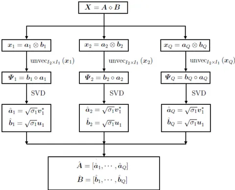
In some applications addressed in this thesis, we will be interested in approxi-mating a matrix Khatri-Rao product between two factor matrices. This problem appears repeatedly over the next chapters in the context of our applications. To solve it, we make use of the well known LS-KRF algorithm proposed by Kinbangou and Favier (2009); Roemer and Haardt (2010); Roemer (2013). In the following, we formulate the Khatri-Rao factorization problem. In addition, the LS-KRF algorithm is summarized in the pseudo-code form.
LetX ∈CI1I2×Qbe an observed data matrix given by the Khatri-Rao product X ≈A⋄B, where A∈CI1×Q and B ∈ CI2×Q. We want to obtain the matrices A and B fromX by solving the following optimization problem:
min
A,BkX −A⋄Bk 2
Algorithm 1 Least-squares Khatri-Rao factorization (LS-KRF) 1: procedure LS-KRF
2: for q= 1, . . . , Q
3: 1. Apply the unvecI2×I1 operator in the q-th column of X to obtain the rank-1 4: matrix Ψq∈CI2×I1 in (14).
5: 2. Compute the SVD of Ψq given by UqΣqVHq. Then, obtain the estimates for 6: the q-th column of Aˆ and Bˆ as follows:
7:
ˆ
aq=√σ1v∗1 and ˆbq =√σ1u1,
8: where u1 and v1 denote the dominant left and right singular vectors of Uq and 9: Vq, and σ1 represents the dominant singular value of Σq,respectively.
10: end
11: The final estimates are given by Aˆ = [ˆa1,· · · ,aQ]ˆ and Bˆ = [ˆb1,· · · ,ˆbQ].
12: Remove the scaling ambiguities of Aˆ and Bˆ through normalization procedure.
According toDefinition 2 and using the property (9), the q-th column ofX can be interpreted as the vectorized form of the following rank-1 matrix
Ψq =bq◦aq ∈CI2×I1, (14)
where aq ∈ CI1 and bq
∈ CI2 denote the q-th column (q = 1, . . . , Q) of A and B, respectively. Therefore, being Ψq ∈ CI2×I1 a rank-1 matrix the best estimates for the vectorsaq and bq in the least squares (LS) sense can be obtained by truncating the SVD of Ψq, defined by UqΣqVHq, to a rank-1 approximation, i.e.,
ˆ
aq =√σ1v∗1 and ˆbq=√σ1u1, (15)
whereu1 and v1 are the dominant left and right singular vectors ofUq andVq, and σ1 is
the dominant singular value of Σq, respectively. Note that the estimated vectors ˆaq and ˆ
bq are affected by non-zero complex scaling ambiguity, i.e.,aq⊗bq = (γq·aq)ˆ ⊗
1
γq ·
ˆ bq. However, it can be easily removed through normalization if the first row of A or B is known (Roemer, 2013). The final estimates ˆA= [ˆa1,· · · ,aQ] and ˆˆ B = [ˆb1,· · · ,ˆbQ] are
obtained by solving this rank-1 approximation problem for each column of X. Based on the aforementioned computational complexity of the rank-1 approximation problem solved via SVD, we can observe that the computational cost of the LS-KRF algorithm is
O(I1·I2·Q).
Figure 1: Schematic of the parallelized procedure for the LS-KRF computation.
Source: Created by the author.
2.3 Tensor Definitions and Operations
The remainder of this chapter is dedicated to presenting the theoric and algo-rithmic concepts of multilinear (tensor) algebra. We begin by introducing some definitions and operations of multilinear algebra. At the end, we provide an overview on the most important tensor decompositions to be used in this thesis, which are the PARAFAC, Nested-PARAFAC and Tucker decompositions.
Throughout this thesis, an N-th order tensor (or higher-order tensor) X ∈
CI1×I2×···×IN with size I
n along mode (or dimension) n (n = 1, . . . , N) and elements
xi1,i2,...,iN is interpreted as a multidimensional array of numerical values with
dimensional-ity N. Mathematically, it represents an element of the tensor product between N vector spaces (Comon, 2014). As special cases matrices, vectors and scalars are commoly referred as 2-order, 1-order and 0-order tensors, respectively. Other definitions and operations in-volving tensors are presented in the following.
Definition 4. (Inner product) The inner product between two tensorsX and Y both of
N-th order, denoted by hX,Yi, results in a scalar value given by
hX,Yi= I1
X
i1=1 I2
X
i2=1
· · ·
IN
X
iN=1
xi1,i2,...,iNyi1,i2,...,iN. (16)
Figure 2: Illustration of a rank-1 third-order tensor. Source: Adapted from
(de Almeida, 2007)
Figure 3: Illustration of the horizontal, lateral and frontal slices of a third-order tensor. Source: Adapted from (de Almeida, 2007)
Definition 5. (Frobenius norm) The Frobenius norm of an N-th order tensor X ∈
CI1×I2×···×IN is defined as
kXkF =
v u u t
I1
X
i1=1 I2
X
i2=1
· · ·
IN
X
iN=1
|xi1,i2,...,iN|2. (17)
The Frobenius norm can be also represented using inner product notation as kXkF = p
hX,Xi. Note that (17) is similar to the matrix Frobenius norm if N = 2.
Definition 6. (Rank-1 tensor) An N-th order tensor X ∈ CI1×I2×···×IN is said to be
rank-1 when it is computed as the outer product betweenN vectors, i.e.,
X =x1◦x2◦ · · · ◦xN, (18)
where xn ∈ CIn (n = 1, . . . , N) is called component of X along the n-th mode (or
dimension). As a visual example, Figure 2 illustrates a rank-1 third-order tensor X ∈
CI1×I2×I3 formed by the outer product of three vectors x
1 ∈CI1, x2 ∈CI2 and x3 ∈CI3.
Figure 4: Construction process of the 1-mode, 2-mode and 3-mode unfolding matrices of a third-order tensor from its frontal, horizontal and lateral slices.
Source: Adapted from (Ximenes, 2015)
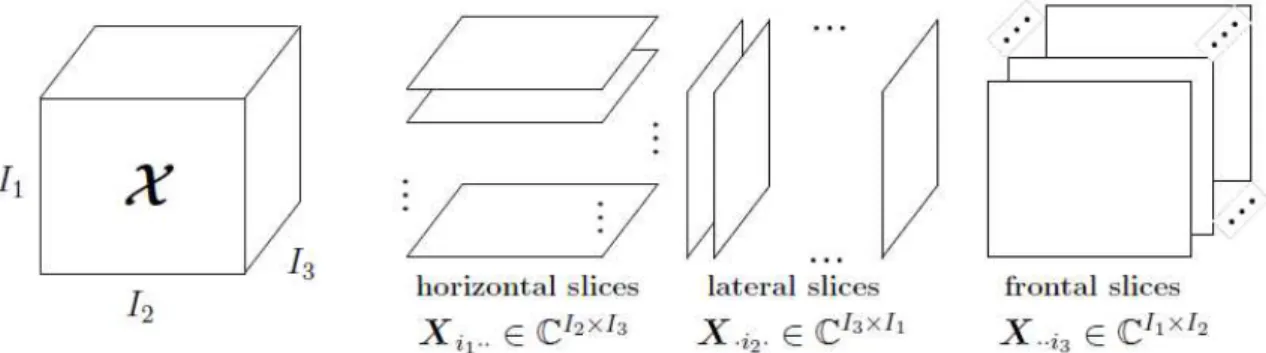
Definition 8. (Fibers) Ann-mode fiber represents an one-dimensional section of a tensor analogue of matrix rows and columns. A fiber is obtained by fixing every index but one. Ann-mode fiber has sizeIn×1, whereIn denotes the size of then-th mode of the tensor. Third-order tensors are formed by row, column and tube fibers (Kolda and Bader, 2009). Definition 9. (Slices) A slice represents a two-dimensional section of a tensor. It is obtained by fixing all but two indices. Third-order tensors are formed by horizontal, lateral and frontal slices as illustrated in Figure 3.
Definition 10. (n-mode unfolding) Then-mode unfolding matrix, represented by [X](n), is the process of reordering the elements of an N-th order tensor X ∈ CI1×I2×···×IN into
of X. Since many computational resources are not able to manipulate tensors of order higher than two, the unfolding matrix concept is important to facilitate the computational manipulation of a given data tensor. Figure 4 illustrates the construction process of the 1-mode [X](1) ∈CI1×I2I3, 2-mode [X]
(2) ∈ CI2×I1I3 and 3-mode [X](3) ∈CI3×I1I2 unfolding
matrices of a third-order tensor X ∈ CI1×I2×I3 from its frontal, horizontal and lateral slices, respectively.
Definition 11. (n-mode product) Then-mode product operation, denoted by×n, consists of multiplying an N-th order tensor X ∈ CI1×I2×···×IN by a matrix A∈ CQ×In along its n-th mode. The result of this operation is
Y =X ×nA∈CI1×I2×···×In−1×Q×In+1×···×IN. (19)
The n-mode product can be also represented in terms of then-mode unfolding matrices of X as follows
[Y](n) =A[X](n). (20)
In other words, then-mode product multiplies all then-mode fibers ofX with the matrix A from the left hand side. In this work, we shall make use of the following n-mode product properties (Kolda and Bader, 2009):
X ×mA×nB=X ×nB×mA (m6=n), (21)
X ×nA×nB=X ×n(BA). (22)
2.4 Tensor Decompositions
This section provides an overview on the main tensor decompositions encoun-tered in the applications investigated throughout this thesis, namely PARAFAC, Nested-PARAFAC and Tucker decompositions.
2.4.1 PARAFAC Decomposition
Figure 5: PARAFAC decomposition ofX ∈CI1×I2×I3 intoQcomponents.
Source: Adapted from (de Almeida, 2007)
Let X ∈ CI1×I2×I3 be a third-order tensor, the PARAFAC decomposition factorizes it into a sum ofQ rank-1 component tensors. i.e.,
X =
Q
X
q=1
a(1)q ◦a(2)q ◦a(3)q , (23)
where its (i1, i2, i3)-th element is given by
xi1,i2,i3 = Q
X
q=1
a(1)i1,qa(2)i2,qa(3)i3,q, (24)
whereQis called number of factors or rank ofX and it is defined as the minimum number of rank-1 tensors for which (23) holds exactly. a(1)i1,q, a(2)i2,q and a(3)i3,q are the elements of the factor matrices A(n) = ha(1n),· · · ,a(Qn)i ∈ CIn×Q (i
n = 1, . . . , In and n = 1,2,3), respectively. Figure 5 illustrates the PARAFAC decomposition of X ∈ CI1×I2×I3 into Q rank-1 components.
The PARAFAC decomposition (23) can be also alternatively represented, in terms of its factor matrices, in a more compact form by using then-mode product notation as follows
X =I3,Q×1A(1)×2A(2)×3A(3), (25)
where I3,Q represents a third-order identity tensor of size Q×Q×Q. The elements of
I3,Q are equal to 1 when all indices are equal, and 0 elsewhere.
As previously mentioned in Section (2.3), we can represent X into three dif-ferent ways according to Definition 9. The horizontal Xi1·· ∈ CI2×I3 (i1 = 1, . . . , I1),
lateral X·i2· ∈ CI3×I1 (i2 = 1, . . . , I2) and frontal X··i3 ∈ CI1×I2 (i3 = 1, . . . , I3) slices of
(25) are denoted by
Xi1·· =
Q
X
q=1 a(1)i1,qa
(2)
q a(3) T
q =A(2)Di1
A(1)
A(3)T, (26)
X·i2·= Q
X
q=1 a(2)i2,qa
(3)
q a(1) T
q =A(3)Di2
Algorithm 2 ALS-PARAFAC 1: procedure ALS-PARAFAC
2: 1. Set i= 0. Randomly initialize Aˆ(2)(i=0) and Aˆ (3) (i=0);
3: 2. i←i+ 1;
4: 3. From [X](1) in (29), obtain an LS estimate of Aˆ(1)(i):
5:
ˆ
A(1)(i) = [X](1)Aˆ((3)i−1)⋄Aˆ(2)(i−1)T
†
;
6: 4. From [X](2) in (30), obtain an LS estimate of Aˆ(2)(i): 7:
ˆ
A(2)(i) = [X](2)
ˆ
A(3)(i−1)⋄Aˆ (1) (i)
T†
;
8: 5. From [X](3) in (31), obtain an LS estimate of Aˆ(3)(i): 9:
ˆ
A(3)(i) = [X](3)Aˆ(2)(i) ⋄Aˆ(1)(i)T
†
;
10: Repeat steps 2-5 until convergence.
X··i3 = Q
X
q=1
a(3)i3,qa(1)q a(2) T
q =A(1)Di3
A(3)A(2)T. (28)
According to Definition 10 and using the property (4) and the expressions (26), (27) and (28), we can express the 1-mode [X](1) ∈CI1×I2I3, 2-mode [X]
(2) ∈CI2×I1I3
and 3-mode [X](3) ∈CI3×I1I2 unfolding matrices of the PARAFAC decomposition as
[X]1 = [X··1· · ·X··I3] =A(1)
h D1
A(3)A(2)T· · ·DI3
A(3)A(2)Ti
=A(1)A(3)⋄A(2)T ∈CI1×I2I3, (29)
[X](2) =XT··1· · ·XT··I3 =A(2)hD1
A(3)A(1)T· · ·DI3
A(3)A(1)Ti
=A(2)A(3)⋄A(1)T ∈CI2×I1I3, (30)
[X](3) = [X·1·· · ·X·I2·] =A
(3)hD 1
A(2)A(1)T· · ·DI2
A(2)A(1)Ti
=A(3)A(2)⋄A(1)T ∈CI3×I1I2. (31)
e(i)= w w w w w w
X −I3,Q×1Aˆ (1) (i) ×2Aˆ
(2) (i) ×3Aˆ
(3) (i)
| {z }
ˆ X(i)
w w w w w w F
, (32)
where ˆX(i)is the reconstructed version ofX computed from the estimated factor matrices
ˆ
A((ni))(n= 1,2,3) obtained at the end of thei-th iteration. δis a prescribed threshold value
assumed to be 10−6 throughout this thesis. The ALS-PARAFAC algorithm is summarized
in Algorithm 2. Note that the dominant cost of the ALS-PARAFAC algorithm is associ-ated with the SVD computation used to calculate three pseudo-inverses in lines 5, 7 and 9 of Algorithm 2. Therefore, the overall computational complexity of the ALS-PARAFAC (per iteration) can be approximated to O(Q2(I1I2+I1I3+I2I3)) FLOPs.
Uniqueness of the PARAFAC Decomposition
The most attractive feature of the PARAFAC decomposition for signal pro-cessing applications is its simple and well defined essential uniqueness property that is guaranteed by the Kruskal’s condition introduced by Kruskal (1977). This condition is based on the following fundamental Kruskal-rank (k-rank) definition:
Definition 12. (k-rank) The Kruskal-rank of A ∈ CI1×Q, defined as κ
A, is the
maxi-mum number such that any subset of κA columns of A are linearly independent. As a
consequence κA ≤ ρA ≤ min (I1, Q), in which ρA denotes the rank of A. If A is a full
rank matrix it is also fullk-rank, i.e.,κA =ρA.
For the third-order tensor (23), if the following Kruskal’s condition is satisfied
κA(1) +κA(2)+κA(3) ≥2Q+ 2, (33)
the uniqueness of its PARAFAC decomposition is guaranteed. Basically, any triplet
ˆ
A(1),Aˆ(2),Aˆ(3) is related to the true triplet A(1),A(2),A(3) up to trivial permu-tation and scaling of columns. In this case, the true and estimated factor matrices are linked by the following relation:
ˆ
A(n)=A(n)Π∆(n), n= 1,2,3, (34)
Extension of the PARAFAC Decomposition to N-th Order Tensors
For simplicity of presentation, we first introduced above only the PARAFAC decomposition of a third-order tensor. However, its generalization for anN-th order tensor is straightforward. The PARAFAC decomposition of the rank-QtensorX ∈CI1×I2×···×IN
is given by
X =
Q
X
q=1
a(1)q ◦a(2)q ◦ · · · ◦a(qN), (35)
or, equivalently, by usingn-mode product notation we get
X =IN,Q×1A(1)×2A(2)· · · ×N A(N). (36)
The n-mode unfolding matrix of (36) is given by
[X](n) =A(n)A(N)⋄ · · · ⋄A(n+1)⋄A(n−1)⋄ · · · ⋄A(1)T. (37)
Remark: Throughout Chapter 3, a special attention is given to dual-symmetric tensors. The PARAFAC decomposition of a tensor X ∈ CI1×···×I2N of even order 2N is
said to have dual-symmetry if it is defined as (Weis, 2015):
X =I2N,Q×1A(1)×2A(2)· · · ×N A(N)×N+1A(1) ∗
×N+2A(2) ∗
· · · ×2N A(N)
∗
, (38)
where IN+n = In and A(N+n) = A(n)
∗
(n = 1, . . . , N). This definition also applies to Tucker decomposition by simply replacing the identity tensor I2N,Q by an arbitrary core tensorG of order 2N.
The generalization of the Kruskal’s condition (33) was formulated by Sidiropou-los and Bro (2000) for an N-th order tensor. For the generalized case, the Kruskal’s condition becomes:
N
X
n=1
κA(n) ≥2Q+ (N −1). (39)
2.4.2 Nested-PARAFAC Decomposition
The Nested-PARAFAC decomposition was introduced and also applied by de Almeida and Favier (2013) in the wireless communication area. The Nested-PARAFAC decomposition assumes that the n-th factor matrix A(n) ∈CIn×Q in (25) is itself an
un-folding matrix of an additional PARAFAC decomposition. By assuming, for simplicity of presentation, that A(1) ∈ CI1×Q denotes the 1-mode unfolding of the third-order tensor
Y ∈ CJ1×J2×J3, i.e., A(1) = [Y]
(1) in which J1 = I1 and J2J3 = Q, we can define the
ˆ A
(i) = [X](1) Aˆ(i−1)⋄Aˆ(i−1) ;
7: 1.4From[X](2),obtain an LS estimate of Aˆ(2)
(i): 8:
ˆ A(2)(
i) = [X](2)
ˆ A(3)(
i−1)⋄Aˆ (1) (i)
T† ;
9: 1.5From[X](3),obtain an LS estimate of Aˆ(3)(i):
10:
ˆ A(3)
(i) = [X](3)
ˆ A(2)
(i)⋄Aˆ (1) (i)
T† ;
11: Repeat steps 1.2-1.5until convergence.
12: Second Stage: ALS-PARAFAC in the inner PARAFAC part
13: 2.1Construct the tensor YfromAˆ(1)= [Y](1);
14: 2.2Set i= 0.Randomly initialize Bˆ(2)
(i=0)and Bˆ (3) (i=0); 15: 2.3i←i+ 1;
16: 2.4From[Y](1),obtain an LS estimate of Bˆ(1)(i):
17:
ˆ B(1)(
i) = [Y](1)
ˆ B(3)(
i−1)⋄Bˆ (2) (i−1)
T† ;
18: 2.5From[Y](2),obtain an LS estimate of Bˆ(2)(
i): 19:
ˆ B(2)
(i) = [Y](2)
ˆ B(3)
(i−1)⋄Bˆ (1) (i)
T† ;
20: 2.6From[Y](3),obtain an LS estimate of Bˆ(3)
(i): 21:
ˆ
B(3)(i) = [Y](3)
ˆ
B(2)(i)⋄Bˆ(1)(i)T †
;
22: Repeat steps 2.3-2.6until convergence.
decompositions
X = I3,Q×1[Y](1)×2A(2)×3A(3), (40) Y = I3,Q×1B(1)×2B(2)×3B(3), (41)
where (40) is called outer PARAFAC part, while (41) is called inner PARAFAC part (Liu et al., 2013). The matrices B(n)∈CJn×Q (n = 1,2,3) are the factor matices of the inner
PARAFAC part. Note that, in a generalized representation form, the inner PARAFAC part may be associated with any mode of X without loss of generality.
Figure 6: Tucker decomposition of a third-order tensorX ∈CI1×I2×I3. Source:
Adapted from (de Almeida, 2007)
can be formulated as two linked PARAFAC decompositions according to (40) and (41), its uniqueness is achieved satisfying together the following two Kruskal’s conditions:
κA(1) +κA(2)+κA(3) ≥2Q+ 2 and κB(1)+κB(2)+κB(3) ≥2Q+ 2. (42)
2.4.3 Tucker Decomposition
The Tucker decomposition was introduced by Tucker (1966). Given a third-order tensorX ∈CI1×I2×I3, the Tucker decomposition factorizes it as a multilinear trans-formation of a third-order core tensor G ∈ CQ1×Q2×Q3 by the factor matrices A(n) = h
a(1n),a(2n), . . . ,aQ(nn)i ∈ CIn×Qn (n = 1,2,3) as illustrated in Figure 6. Mathematically,
the Tucker decomposition ofX is defined as
X =
Q1
X
q1=1 Q2
X
q2=1 Q3
X
q3=1
gq1,q2,q3 a
(1)
q1 ◦a(2)q2 ◦a(3)q3
, (43)
where its (i1, i2, i3)-th element is given by
xi1,i2,i3 = Q1
X
q1=1 Q2
X
q2=1 Q3
X
q3=1
gq1,q2,q3a
(1)
i1,q1a
(2)
i2,q2a
(3)
i3,q3, (44)
where Qn is the multilinear rank of X, i.e., the number of components in the n-th (n = 1,2,3) mode of X. a(inn,q)n is the (in, qn)-th element of the factor matrix A
(n)
∈ CIn×Qn
(n = 1,2,3) and gq1,q2,q3 is the (q1, q2, q3)-th element of the core tensor G ∈ C
Q1×Q2×Q3. Using then-mode product notation, the Tucker decomposition ofX can be written as
[X](3) =A(3)[G](3)A(2)⊗A(1)T, (48)
where [G](1) ∈ CQ1×Q2Q3, [G]
(2) ∈ CQ2×Q1Q3 and [G](3) ∈ CQ3×Q1Q2 denote the 1-mode,
2-mode and 3-mode unfolding matrices of G, respectively. The Tucker2 decomposition where A(3) =II3 and G ∈CQ1×Q2×I3, and the Tucker1 decomposition where A(3)
=II3, A(2) =II2 and G ∈ CQ1×I2×I3 are special cases of the Tucker decomposition (Kolda and Bader, 2009).
Uniqueness of the Tucker Decomposition
In general, the Tucker decomposition is not unique i.e., there are infinite solu-tions for the factor matrices and for the core tensor that leads to the same tensor X. Proof. LetT(n) (n = 1,2,3) be non-singular matrices, we can rewrite (45) as
X = ˆG×1Aˆ(1)×2Aˆ (2)
×3 Aˆ (3)
=G×1T(1) −1
×2 T(2) −1
×3T(3) −1
| {z }
ˆ G
×1A(1)T(1) | {z }
ˆ A(1)
×2A(2)T(2) | {z }
ˆ A(2)
×3A(3)T(3) | {z }
ˆ A(3)
=G×1T(1) −1
×1 A(1)T(1)×2T(2) −1
×2 A(2)T(2)×3T(3) −1
×3A(3)T(3).
Making use of the property (22), we obtain
X =G×1A(1)T(1)T(1)−1×2
A(2)T(2)T(2)−1×3
A(3)T(3)T(3)−1
=G×1A(1)×2A(2)×3A(3).
Extension of the Tucker Decomposition to N-th Order Tensors
For anN-th order tensorX ∈CI1×I2×···×IN, itsN-th order Tucker
decomposi-tion is given by
X =
Q1
X
q1=1 Q2
X
q2=1
· · ·
QN
X
qN=1
gq1,q2,...,qN a
(1)
q1 ◦a(2)q2 ◦ · · · ◦a( N)
qN
, (49)
or, equivalently, by usingn-mode product notation
X =G×1A(1)×2A(2)· · · ×N A(N). (50)
The n-mode unfolding matrix of (50) is given by
[X](n) =A(n)[G](n)A(N)⊗ · · · ⊗A(n+1)⊗A(n−1)⊗ · · · ⊗A(1)T. (51)
The Higher-Order Singular Value Decomposition (HOSVD)
The HOSVD, introduced by Lathauwer, Moor, and Vandewalle (2000), is a direct extension of the matrix SVD to higher-order tensors. It is a way to compute the basis for each factor matrix of the Tucker decomposition. The HOSVD of an N-th order tensorX ∈CI1×I2×···×IN is defined as
X =S ×1U(1)×2U(2)· · · ×N U(N), (52)
where U(n) ∈ CIn×Qn (n = 1,2, . . . , N) are unitary matrices and S ∈ CQ1×Q2×···×QN is
the core tensor. The set (Q1, Q2, . . . , QN) denotes the multilinear rank ofX. The matrix U(n) is computed as the Qn left singular vectors of the n-th unfolding matrix of X, i.e.,
[X](n) =U(n)Σ(n)V(n)H. (53)
FromU(n) (n= 1,2, . . . , N) computed according (53), the core tensor can be obtained as
S =X ×1U(1)H×2U(2)
H
· · · ×N U(N) H
. (54)
The HOSVD procedure is described in the pseudo-code form in Algorithm 4.
5: end
6: 2. Compute the core tensor as: 7:
S =X ×1U(1)H ×2U(2)
H
· · · ×N U(N) H
.
8: 3. Return S and U(n) (n = 1,2, . . . , N).
2.5 Chapter Summary
3 TENSOR-BASED METHODS FOR BLIND SPATIAL SIGNATURE ES-TIMATION IN MULTIDIMENSIONAL SENSOR ARRAYS
In this chapter, we address the spatial signatures and spatial frequencies estimation prob-lems in multidimensional (R-D) sensor arrays. It is divided into two parts. In the first part of this chapter, we propose a tensor-based multiple denoising approach that succes-sively applies spatial smoothing, denoising and reconstruction to the noisy data. By taking into account the knowledge of the model order and by exploiting subarrays created by the spatial smoothing, we can successively denoise the data by means of HOSVD-based and SVD-based low-rank approximation for tensor and matrix data, respectively. In the second part of this chapter, we propose two generalized iterative algorithms for spatial signatures estimation. The first tensor-based algorithm is an R-D blind spatial signature estima-tor that operates in scenarios where the sources’ covariance matrix is nondiagonal and unknown. The second tensor-based algorithm is formulated to address the uncorrelated sources case and exploits the dual-symmetry of the covariance tensor. Additionally, a new tensor-based formulation is proposed for an L-shaped array configuration. Simula-tion results show that the proposed receiver, referred to as multiple denoising (MuDe), significantly reduces the noise level, yielding a more accurate estimation of the parameters without decreasing the sensor array aperture, while the algorithms proposed in the sec-ond part outperform the state-of-the-art matrix-based and tensor-based spatial parameter estimation techniques.
3.1 Introduction and Motivation
The high resolution parameter estimation from noisy signal measurements plays a key role in several practical applications in the array signal processing area rang-ing from MIMO communications (Zhou et al., 2016a), radar (Singh, Wang, and Crag´e, 2016; Nion and Sidiropoulos, 2010) and global navigation satellite systems (GNSS) (Ham-moudet al., 2016) to name a few. The performance of parameter estimation techniques is sensitive to the SNR and severely degrades in noisy scenarios. Therefore, a denoising pre-processing can be an effective step to improve the SNR and consequently the estimation accuracy.
performance can be achieved by exploiting the multidimensional structure of the data by means of tensor modeling, which can include several signal dimensions such as space, time, frequency, and polarization. Tensor decompositions have been successfully employed in array signal processing for parameters estimation since they provide better identifiability conditions when compared to conventional matrix-based techniques. Another advantage of tensor-based methods is the so-called tensor gain which manifests itself with more precise parameter estimates due to the good noise rejection capability of tensor-based signal processing as shown in (da Costaet al., 2011; Roemer, 2013; da Costa et al., 2013; da Costa, 2010).
In this chapter, we address the spatial signatures and spatial frequencies esti-mation problems in multidimensional sensor arrays. In the first part of the chapter, we show that, by taking into account the model order and by exploiting the possible subar-rays created by the spatial smoothing, the data can be successively denoised by means of the HOSVD-based and SVD-based low-rank approximations, which drastically reduces the noise effect in tensor and matrix data, respectively. We initially propose a new tensor-based preprocessing method for noise reduction in noisy measurement data collected by a multidimensional (R-D) sensor array. Exploiting the spatial smoothing concept (Shan, Wax, and Kailath, 1985), a better signal estimation is obtained by applying successive SVD-based low-rank approximations in the output signals for subarrays of different sizes in each spatial dimension of the received signal tensor, and then reconstructing back the subarrays into the original tensor so that the procedure can be repeated. We also discuss the matrix-based approach that is a particular case of the proposed method when an one-dimensional sensor array is considered.