Feedback Reduction of Spatially Multiplexed
MIMO Systems Using Compressive Sensing
Raymundo Nogueira de S´a Netto and Charles Casimiro Cavalcante
Abstract— In this paper we analyze spatially multiplexed
MIMO systems with limited Channel State Information (CSI) and zero forcing (ZF) linear signal detection technique. Two schemes were considered: Quantization Codebook (QC) and Compressive Sensing (CS). Compressive Sensing is used to generate a reduced CSI feedback to the transmitter in order to reduce feedback load into the system. Performance of the schemes are compared by computational simulations of bit error rate (BER) curves for the considered approaches QC and CS.
Keywords— BER, limited feedback, compressive sensing,
quan-tization codebook.
I. INTRODUCTION
Spatially multiplexed MIMO (SM-MIMO) systems can transmit data at higher speed than MIMO systems using antenna diversity techniques [1]. Zero Forcing (ZF) is one of the techniques we could use for signal detection in those systems. It needs complete Channel State Information (CSI) knowledge and a way to acquire it is using a feedback link from the receiver. However, even if the CSI can be perfectly estimated at the receiver, the required bandwidth for feedback is aggravated as the number of transmit and receive antennas increases [2]. Limited feedback beamforming is used to reduce the required bandwidth. When implemented, the beamforming vector is restricted to lie in a finite set or codebook that is known to both the transmitter and receiver [3].
Recently, Compressive Sensing (CS), also known as com-pressed sensing or compressive sampling, has been applied in diverse contexts of signal processing and communications, where the information content is sparse [3]. The spatial correlation between antenna arrays was exploited in [2] in order to obtain sparse representations of the channel and use CS to reduce the feedback load. CS is used in [4] to reduce the requirement of memory and complexity as the feedback rate increases and achieve greater sum throughput compared to Vector Quantization Codebook (VQC). In [5] it was proposed the use of CS to reduce the feedback for digital and analog schemes to achieve the same sum-rate throughput as the one achieved by dedicated feedback schemes, with limited feedback channels. Users that have a SINR larger than a threshold transmit the same feedback information and they are identified by the Base Station (BS) using CS and also a relation between sparsity and the threshold was given in [8]. In [9] a distributed self-selection procedure is combined with CS to identify a set of users who are getting simultaneous access to the downlink broadcast channel.
Raymundo Nogueira de S´a Netto and Charles Casimiro Cavalcante¸ Depar-tamento de Engenharia de Teleinform´atica, Universidade Federal do Cear´a, Fortaleza-CE, Brasil, E-mails: [email protected], [email protected].
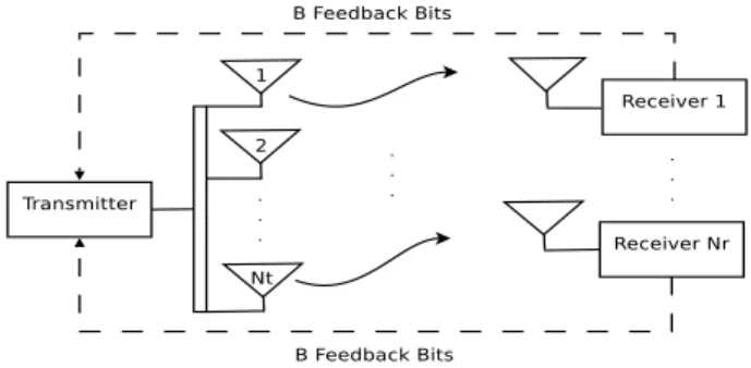
Fig. 1. Limited feedback system model
This work is based on [4], but instead of comparing the sum throughput between CS and VQC feedbacks, it uses CS to reduce the feedback load and to do a comparison between CS or VQC, both with limited feedback, and ZF technique with full CSI. This comparison has been made for two spatially multiplexed MIMO systems and the element of analysis is the Bit Error Rate (BER) over a Signal-to-Noise Ratio (SNR) variation.
The remainder of this paper is organized as follows. Section II provides the system model, as well as a review of CS operation. Section III shows how the feedback load reduction occurs. The results obtained by the two feedback protocols are shown in Section IV. Finally, in Section V, our conclusions are stated.
II. SYSTEMMODEL
We consider MIMO wireless communication system with
Nt transmit antennas and Nr receive antennas, as shown in
Figure 1. The received signal vector at the Nr antennas is
written as
y=Hx+n, (1)
whereH= [h1,h2, ...,hNt]
T
is the channel matrix with inde-pendent and identically distributed (i.i.d) complex zero-mean
unit variance Gaussian random values,nis an additive white
Gaussian noise (AWGN) and x is the precoded vector that
satisfies an average transmit power constraintE{xHx}= 1,
where E={.} is the expectation operator and ()H is the
conjugate transpose..
detection of desired signals from each antenna, the effect of
the channel is inverted by a weight matrixW such that
y=HWx+n, (2)
whereWin ZF technique is defined by
W= (HHH)−1HH, (3)
where (.)H denotes the Hermitian transpose operation. W
is calculated at the receivers and they feed it back to the
transmit antennas, i.e.,Wrepresents the CSI. For our purposes
it has been considered that Wcan be perfectly estimated at
the receivers and the feedback channel is noiseless and delay free. However, as shown in Figure 1, the feedback channel is limited, so the CSI is not completely obtained by the transmit antennas. Thus, BER is not the same as the one considering ZF technique with full CSI. In this work, we assume the limited feedback channel has two protocols being used: quantization codebook (QC) and compressive sensing.
A. Quantization Codebook
In a limited feedback channel each receive antenna
quan-tizes its channel using B bits and feeds back these bits.
The quantization is performed using a vector quantization codebook that is known at the transmit and receive antennas. Typically, each receive antenna uses a differente codebook to prevent multiple antennas from quantizing their channel to the same quantization vector [4]. A quantization codebook
C = {c1, ...,c2B} consists of 2B codeword vectors. Each
codeword vector ci has unit norm and length equal to the
number of transmit antennas Nt.
The receive antenna quantizes its channel to the quantization vector (codeword) that is closest to its channel vector. This closeness is measured in terms of the angle between two vectors or, equivalently, the inner product [4]. Thus, a receive
antennai obtains the quantization indexFi according to [3]
Fi= arg max j=1,...,2B|h
H i cj| = arg min
j=1,...,2Bsin 2(6 (h
i,cj)),
(4)
and feeds this index back to the transmit antenna. The choice of vector quantization codebook significantly affects the qua-lity of the CSI provided to the transmit antenna, i.e., the larger is the codebook the better is the quality of the CSI.
B. Compressive Sensing
Before explaining how CS is used on a limited feedback scheme, a brief overview is shown. This emerging theory is based on exploiting the sparsity present into the signals, being able to recover these signals from a limited number of linear measurements, and it is more effective compared to the classical Nyquist-Shannon sampling [5], [11]. Sparsity expresses the idea that the “information rate” of a continuous time signal may be much smaller than suggested by its bandwidth, or that a discrete-time signal depends on a number of degrees of freedom which is comparably much smaller than its (finite) length. More precisely, CS exploits the fact that many natural signals are sparse or compressible in the sense
that they have concise representations when expressed in a
proper basisA [6].
Letxbe aN×1vector, with at mostSnon-zero elements,
whereS << N. Consider aM ×N measurement matrixA,
where M << N and M > S. The measurements can be
obtained by
b=Ax, (5)
where b is a M ×1 vector. Since M << N the vector x
can be represented bybwith much less information, i.e.,xis
compressed intob.
Hence, this system has more unknowns than equations, and
thus it has either no solution, if b is not in the span of the
columns of the matrix A, or infinitely many solutions. To
avoid these conditions to happen,Ahas to havel2-normalized
columns, and for an integer scalar s ≤ n, consider
sub-matrices As containing s columns from A. δs is defined as
the smallest quantity such that
∀x∈Rs: (1−δs)||x||22 ≤ ||Asx||22≤(1 +δs)||x||22, (6)
holds true for any choise ofscolumns. ThenAis said to have
ans-restricted isometry property (RIP) with a constantδs[11].
This constant measures how orthonormally close the column
vectors of the measurement matrix Aare to each other.
On the other side, a recovery algorithm has to be used to
obtainx from b. If the RIP holds, then the following linear
program gives an accurate reconstruction [10]:
min
x∈Rn||x||l1 subject to Ax=b. (7)
To solve this optimization task, there are some proposed
algorithms on literature:l1-Magic [12], Orthogonal Matching
Pursuit (OMP) [13], Basis Pursuit (BP) [14], Dantzig-Selector
(DS) [11].
Returning to our purpose, we desire to compress the CSI
to reduce the feedback load. According to H features, it is
not sparse to use CS for compression. Song et al. proposed a CSI sparse approximation method [4]. Like the quantization
codebook, aNt×2B matrixQ= [q
1. . .qm. . .q2B], called
dictionary, is required. After this, the method consists of three steps:
1) Column Selection: S columns maximally correlated
with their own CSI (h) are selected. Let π(i) be
the ith column index largely correlated with the
channel vector. Each receive antenna selects the co-lumn maximally correlated from the initial coco-lumn
index set Λ0 = {1, ..., m, ...,2B} of Q as π(1) =
arg maxm∈Λ0|hqm,hi|, where h,i stands for the inner
product, and |.| stands for the absolute value. After
selectingi−1columns, theith column can be selected
within Λi−1 ={m|m ∈ Λi−2 andm 6=π(i−1)} as
π(i) = arg maxm∈Λi−1|hqm,hi|. This continues until
the S columns are selected. Π(i) = {π(1), ..., π(S)}
is the index set for the selected columns. Since this
procedure can find the S-dimensional subspace
maxi-mally correlated tohover theNt-dimensional complex
2) CSI Approximation: Each receive antenna channel
vec-torhis aproximated by the selected S columns in the
minimum-mean-square-error sense, as follows:
z(Π) = arg min
a(Π)||h−Q(Π)a(Π)|| 2
=Q(Π)†h= (Q(Π)HQ(Π))−1Q(Π)Hh, (8)
where ||.|| is the Frobenius norm, ()† is the
pseu-doinverse, Q(Π) is the Nt×S matrix consisting of
column vectors corresponding toΠ,z(Π)is the optimal
coefficient vector for Q(Π), and a(Π) is a candidate
vector forz(Π).
3) Sparse CSI creation: The 2B ×1 sparse CSI can be
obtained as follows:
˜
h=Q(Π)z(Π) =Qz. (9)
In the first equality, the fact thatQ(Π)andz(Π)depend
onΠmakes it difficult to design a universal compression
matrix, which does not depend on the channel vector. To design the given universal compression matrix, we
must redefine ˜h in the second equality of (9) with Q
being independent ofΠandzonly containingSnonzero
elements corresponding toΠ.
Thus, z is S-sparse and CS can be used to compress this
information to be feedback to the transmit antennas
b=Az, (10)
whereAis aM×2Bmeasurement matrix,zcan be recovered
by one of the algorithms previously mentioned, at the transmit
antennas, andhcan be estimated byh=Qz.
So, the difference between quantization codebook and com-pressive sensing is that the transmit and receive antennas in
quantization codebook has to know the codebook C used at
each antenna. On the other hand, in compressive sensing they
has to know the dictionaryQand the measurement matrixA.
III. FEEDBACKLOADREDUCTION
For our studies, it was considered two spatially multiplexed
MIMO systems. The first one has Nt = Nr = 4 and the
second Nt = Nr = 8. The sparsity value S = 1 was the
same for both systems. When we simulated theNt=Nr= 8
system, to sparsify the 8×8 channel matrix H we had to
divide it into four 4×4 matrices to use the same sparsity
value and the number of measurementsM as the first system
(Nt=Nr= 4) and obtain the same feedback load reduction.
S can be recovered with high probability as long as M is
sufficiently large andAsatisfies RIP [10]. SinceAis an i.i.d
Gaussian matrix, according to [8] M has to satisfy
M ≥kSlog2(Nt/S), (11)
wherek is a constant. Consideringk= 1, we obtainM = 2,
which is used at all simulations.
Defined these parameters, the feedback load reduction is calculated for the two systems utilized. We have the following
example that works for every value ofB bits:
a11 a12 . . . a12B
a21 a22 . . . a22B
011 .. .
z
.. .
012B
T
=
b11
b21
, (12)
where (12) is the matrix representation of (10). Since S =
1, z contains only one non-zero element and this sparse
representation can be compressed intoM = 2measurements,
equal to the length ofb. ConsideringNt=Nr= 4, it means
thatH= [h1,h2,h3,h4]T and eachhcan be compressed into
b. So the necessary feedback load for this case is represented
by the following matrix representation:
B=
b11 b12 b13 b14
b21 b22 b23 b24
. (13)
This feedback load is smaller than the one used by the
quan-tization feedback, since each vectorhhas to be representated
by one codeword c and its length is Nt. So, the feedback
load necessary by quantization feedback, in this case, is 32 and the one necessary by compressive sensing is 16, which is represented by each value of (13). It means that, utilizing compressive sensing, the feedback load can be reduced to half of the one used by quantization feedback. It is according to the compression ratio equation provided by [2]:
η=TM/(NTNR), (14)
whereTM represents the total number of measurements. The
same compression ratio (η) is obtained when Nt=Nr = 8,
since, as explained before, each receive antenna separate in
two 4×1 vectors the8×1 CSI vector calculated at it.
IV. RESULTS
The results were obtained considering the ZF technique model using 4-QAM modulation provided by [1] with some adaptation to the feedback limitation and it also provided the codebook design parameters which are the same in IEEE 802.16e specification. All results show the BER variation as SNR increases between the two protocols discussed before for limited feedback and the same variation for ZF, but with full
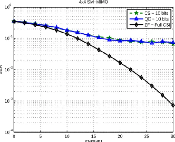
CSI. Considering B = 10 bits, Nt =Nr = 4 and the other
parameters already defined at section III , the first result is shown in Figure 2.
In order to evaluate if the feedback load reduction was going to harm the BER, Figure 2 shows that, for a dictionary in CS with the same length of the codebook in QC, there is no degradation in terms of BER, i.e., they show the same behavior. Comparing both limited feedback schemes to ZF with full CSI, their behaviors is very different. At ZF as long as SNR increases, BER decreases. Otherwise, at the two schemes, the decaiment of BER is worst than the first and it tends to stabilize even if SNR increases.
0 5 10 15 20 25 30 10−4
10−3 10−2 10−1
100
SNR[dB]
BER
4x4 SM−MIMO
CS − 10 bits QC − 10 bits ZF − Full CSI
Fig. 2. BER vs SNR for the three schemes utilized withB= 10bits and
4×4SM-MIMO.
codebook lengths. This second result was obtained utilizing
B = 13bits and is shown in Figure 3.
0 5 10 15 20 25 30
10−4 10−3 10−2
10−1 100
SNR[dB]
BER
4x4 SM−MIMO
CS − 13 bits QC − 13 bits ZF − Full CSI
Fig. 3. BER vs SNR for the three schemes utilized withB= 13bits and
4×4SM-MIMO.
Figure 3 shows that utilizing B = 13 bits a better
appro-ximation to ZF with full CSI is achieved, but, even with this performance increase, the limited feedback schemes continue tending to stabilize, at this time with lower BER and higher SNR, showing the advantage of using more bits. This tendency
continues for every raise in the number of bitsB. Comparing
only CS and VQ, they obtain the same BER variation.
From now on, the results obtained were considering Nt=
Nr= 8, and the other parameters were kept the same. So, for
B = 10andB = 13bits the relation BER vs SNR is shown,
respectively, in Figures 4 and 5.
In Figures 4 and 5 BER exhibit the same behavior presented on Figures 2 and 3, respectively. Comparing CS and QC, BER variation is the same and increasing the number of bits, it was obtained a better approximation to ZF with full CSI for both limited feedback schemes.
The advantage of using CS is shown over all the results over the obtained feedback load reduction in terms of BER compared to QC, since they always have the same BER
0 5 10 15 20 25 30
10−3 10−2 10−1 100
SNR[dB]
BER
8x8 SM−MIMO
CS − 10 bits QC − 10 bits ZF − Full CSI
Fig. 4. BER vs SNR for the three schemes utilized withB= 10bits and
8×8SM-MIMO.
0 5 10 15 20 25 30
10−3
10−2 10−1 100
SNR[dB]
BER
8x8 SM−MIMO
CS − 13 bits QC − 13 bits ZF − Full CSI
Fig. 5. BER vs SNR for the three schemes utilized withB= 13bits and
8×8SM-MIMO.
behavior. Otherwise, the amount of required memory and the computational complexity, as shown in Table I, is higher than in QC. Note that one complex value is saved by a double-precision floating point (64bits/value).
V. CONCLUSIONS
TABELA I
COMPARISON OF THE AMOUNT OF REQUIRED MEMORY AND THE
COMPUTATIONAL COMPLEXITY.
Compressive Sensing Quantization Codebook
Amount of required memory
64×Nt×2B
| {z }
dictionary
+ 64×C×2B
| {z }
measurement matrix
64×Nt×2B
| {z }
codebook
Computational complexity
S×Nt×2B
| {z }
max. correlation
+ S×C
| {z }
compression
+Nt3+S(Nt2+Nt)
| {z }
sparse approximation
Nt×2B | {z }
max. correlation
ACKOWNLEDGMENT
This work was supported by the Brazilian agencies CNPq and FUNCAP/PRONEX.
REFERENCIASˆ
[1] Y. S. Cho, J. Kim, W. Y. Yang and C. Kang, MIMO-OFDM Wireless
Communications with MATLAB. Wiley, 2010.
[2] P. Kuo, H. T. Kung and P. Ting, Compressive Sensing Based Channel
Feedback Protocols for Spatially-Correlated Massive Antenna Arrays.
IEEE Wireless Communications and Networking Conference (WCNC), 2012.
[3] C. K. Au-Yeung and D. J. Love, On the Performance of Random Vector
Quantization Limited Feedback Beamforming in a MISO System. IEEE
Transactions on Wireless Communications, 2007.
[4] H. Song, W. Seo, and D. Hong, Compressive Feedback Based on Sparse
Approximation for Multiuser MIMO Systems. IEEE Transactions on
Vehicular Technology, 2007.
[5] S. T. Qaseem and T. Y. Al-Naffouri, Compressive Sensing for Feedback
Reduction in MIMO Broadcast Channels. IEEE Transactions on Wireless
Communications, April, 2009.
[6] E. J. Candes and M. B. Wakin, An Introduction to Compressive
Sam-pling. IEEE Signal Processing Magazine, March, 2008.
[7] N. Jindal, MIMO Broadcast Channels With Finite-Rate Feedback. IEEE Transactions on Information Theory, November, 2006.
[8] K. Kim, S. Jang and D. Kim, An Efficient Feedback Scheme Using
Compressive Sensing for MIMO Broadcast Channel with Random Beamforming. The 2nd International Conference on Computer and
Automation Engineering (ICCAE), 2010
[9] S.R. Bhaskaran, L. Davis, A. Grant, S. Hanly and P. Tune An
Effici-ent Feedback Scheme Using Compressive Sensing for MIMO Broad-cast Channel with Random Beamforming. IEEE Information Theory
Workshop on Networking and Information Theory, 2009. ITW 2009. [10] E. Candes, J. Romberg and T. Tao, Robust Uncertainty Principles: Exact
Signal Reconstruction from Highly Incomplete Frequency Information.
IEEE Trans. Inf. Theory, vol. 52, no. 2, pp. 489-509, Feb. 2006. [11] M. Elad, Sparse and Redundant Representations - From Theory to
Applications in Signal and Image Processing. Springer, 2010.
[12] E. J. Candes and J. Romberg, l1-MAGIC: Recovery of Sparse Signals via Convex Programming, 2005. Available at http://www.acm.caltech.edu/l1magic.
[13] J. A. Tropp and A. C. Gilbert, Signal recovery from partial information
via Orthogonal Matching Pursuit. IEEE Trans. Inform. Theory, April,
2005.
[14] S. S. Chen, D. L. Donoho, and M. A. Saunders, Atomic decomposition
by Basis Pursuit. SIAM Review, 43(1):129-159, 2001.
[15] D. L. Donoho, Compressed Sensing. IEEE Trans. Inform. Theory, vol. 52, no. 4, pp. 1289-1306 April, 2006.
[16] J. Haupt, W. U. Bajwa, M. Rabbat and R. Nowak, Compressed Sensing