Mobility Data under Analysis a Complex Network Perspective from Interactions Among Trajectories to Movements among Points Interest

(1)

Universidade Federal do Ceará

Departamento de Computação

Curso de Ciência da Computação

Igo Ramalho Brilhante

Mobility data analysis under a complex network perspective:

from interactions among trajectories to movements among points

of interest

(2)

Igo Ramalho Brilhante

Mobility data analysis under a complex network perspective:

from interactions among trajectories to movements among points

of interest

Dissertação submetida à Coordenação do Curso de Pós-Graduação em Ciência da Computação da Universidade Federal do Ceará, como requisito parcial para a obtenção do grau de Mestre em Ciência da Computação.

Área: Ciêcia da Computação

Orientador:Prof. Dr. José Antonio Fernan-des de Macêdo

Coorientadora:Profa. Dra. Chiara Renso

Fortaleza, Ceará

(3)

A000z Brilhante, R. I.

Mobility data analysis under a complex network per-spective: from interactions among trajectories to move-ments among points of interest / Igo Ramalho Brilhante. 2012.

104p.;il. color. enc.

Orientador: Prof. Dr. José Antonio Fernandes de Macêdo Coorientadora: Profa. Dra. Chiara Renso

Dissertação(Ciência da Computação) - Universidade Fed-eral do Ceará, Departamento de Computação, Fortaleza, 2012.

1_. 2_. 3_. _{I. Prof. Dr. José Antonio Fernandes de} Macêdo(Orient.) II. Universidade Federal do Ceará– Ciência da Computação(Mestrado) III. Mestre

(4)

MOBILITY DATA ANALYSIS UNDER A COMPLEX NETWORK PERSPECTIVE: FROM INTERACTIONS AMONG TRAJECTORIES TO

MOVEMENTS AMONG POINTS OF INTEREST

Igo Ramalho Brilhante

Dissertação apresentada ao Curso de Mestrado em Ciência da Computação da Universidade Federal do Ceará, como parte dos Requisitos para a obtenção do Grau de Mestre em Ciência da Computação do aluno Igo Ramalho Brilhante

Composição da Banca Examinadora:

________________________________________________________ Prof. Dr. José Antônio Fernandes de Macedo (Presidente) (DC/UFC)

_____________________________________ Prof. Dr. Marco Antonio Casanova (PUC/Rio)

________________________________ Profa. Dra. Chiara Renso (CNR/Itália)

______________________________________ Profa.Dra. Vânia Maria Ponte Vidal (DC/UFC)

(5)

(6)

(7)

“O único lugar onde o sucesso vem antes do trabalho é no dicionário.”

(8)

Abstract

The explosion of personal positioning devices like GPS-enabled smartphones has enabled the collection and storage of a huge amount of positioning data in the form oftrajectories. Thereby, trajectory data have brought many research challenges in the process of recovery, storage and knowledge discovery in mobility as well as new applications to support our society in mobility terms.

Other research area that has been receiving great attention nowadays is the area of complex network or science of networks. Complex network is the first approach to model complex system that are present in the real world, such as economic markets, the Internet, World Wide Web and disease spreading to name a few. It has been applied in different field, like Computer Science, Biology and Physics. Therefore, complex net-works have demonstrated a great potential to investigate the behavior of complex systems through their entities and the relationships that exist among them.

The present dissertation, therefore, aims at exploiting approaches to analyze mobility data using a perspective of complex networks. The ﬁrst exploited approach stands for the trajectories as the main entities of the networks connecting each other through a similarity function. The second, in turn, focuses on points of interest that are visited by people, which perform some activities in these points. In addition, this dissertation also exploits the proposed methodologies in order to develop a software tool to support users in mobility analysis using complex network techniques.

(9)

List of Figures

Figura 2.1 Example of a trajectory sample whose identiﬁer is 223: (a) interpo-lation between the points; (b) “raw” data of the trajectory, the triples htrajid, xi, yi, tii . . . 25

Figura 2.2 (left) trajectories and (right) trajectories with geographic information [Alvares et al., 2007b]

Figura 2.3 (a) a trajectory moving from left to right and (b) the same trajectory, but with semantic location associated with it. Besides of considering the passing through a location, the time spent on the place can be considered 26

Figura 2.4 Example of application with three candidate stops (RC1, RC2, RC3). Imag-ine a trajectory sample running through from left to right and t0, . . . , t18 are the time points of T. First, T is outside any candidate stop, so it starts a move. Then T enters RC1 at time t1 such that the duration is long enough, t6−t1 ≥ ∆C, then (RC1, t1, t6) is the ﬁrst stop. When the trajectory enters RC2, it do not spend time enough inside that candidate, so it is not a stop. We then have a move until T enters RC3, which fulﬁlls the requests to be a stop, and so (RC1, t1, t6) is the second stop ofT. The trajectory ends with a move [Alvares et al., 2007a] . . . 29

(10)

Figura 3.5 A random graph Gn,p generated with n = 100 and p= 0.05. Its average

shortest path is 2.271 and its clustering coeﬃcient is 0.099 (145 triangles) . . . 40

Figura 3.6 The small world model varying p. This ﬁgure illustrates well the network structure by varying the probabilityp: p= 0 generates a regular network, while p= 1 generates a random network [Watts & Strogatz, 1998] . . . 41

Figura 3.7 A WS network shaping a ring generated with n = 100 and p = 0.2 and

k = 10. Its average shortest path is 2.548 and its clustering coeﬃcient is 0.419 (624 triangles) . . . 42

Figura 3.8 A BA network generated withn = 100andm0 = 4andk= 2. The largest and red nodes represent the preferential attachments, highly connected nodes, which are more likely to establish new links with other nodes . . 43

Figura 3.9 An example of community discovery by perfoming the method proposed

in [Blondel et al., 2008]. This algorithm is available in Gephi [Bastian et al., 2009]. This network was built from a user’s proﬁle in a social network and, thus,

each community represented by a color shows a community of people. For instance, the blue community represents the friends from the university and the red one represents the family ties . . . 44

Figura 4.1 A plotted complex network composed by 36,824 nodes and 306,572 edges generated in our experiments . . . 50

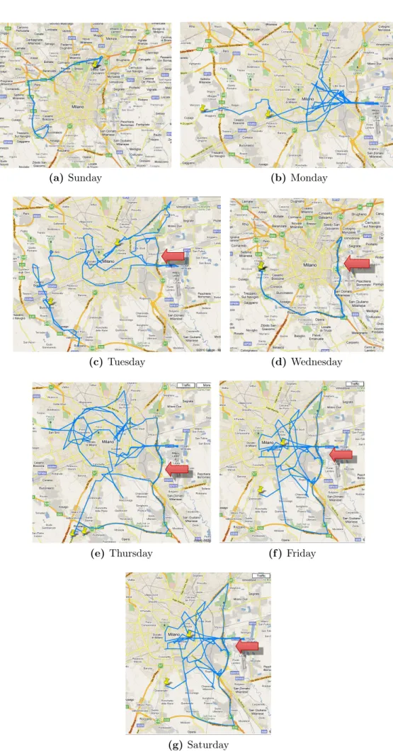
Figura 4.3 Plot showing the number of trajectories for each day of the week . . . 58

Figura 5.1 The building process of places network from one user history: From posi-tional observations in (a) to the user history in (b), the candidates stops in (c). The trajectories set in shown in (d) where a move of duration of 8h30’ (thus exceeding 4 hrs) splits the user history into two trajectories. The POI network is depicted in (e) . . . 70

(11)

Figura 5.3 Edge weight distribution of the networkPN

oi . . . 74

Figura 5.4 The 109 communities discovered from the POIs network. The edge color identify the diﬀerent communities . . . 75

Figura 5.5 Community size distribution considering number of edges. Many commu-nities are formed by a few edges, whereas a few commucommu-nities are composed by a higher number of edges . . . 76

Figura 5.6 Cumulative Distribution ofCompactness. P(Compactness≤k)indicates the probability that Compactness takes on a value less than or equal to

k . . . 76

Figura 5.7 Correlation . . . 77

Figura 5.8 The selected communities: the three largest communities by the number of edges are 72, 20, 25; and the two communities 76 and 63 act like a "bridge" between them characterizing the movement between two regions of the city . . . 78

Figura 5.9 Temporal analysis of the network PN

oi and communities 72, 20 and 25

showed in Figure 5.8 . . . 80

Figura 5.10 Communities to illustrate the measureCompactnessconsidering diﬀerent degrees of compactness: communities 104, 86 and 43 are less compact communities; 6 and 13 are more compact communities . . . 81

Figura 6.2 Statistical analysis performed by M-Atlas: movement distribution (top), cumulative lengths distribution (left) and density of length over speed (right) [Trasarti et al., 2010] . . . 87

(12)

Figura 6.4 NWB interface with the menu to compute network analysis on diﬀerent types of networks, such as node degree, degree distribution, clustering coeﬃcient and community detection . . . 89

Figura 6.5 Interface of Gephi showing the Data Laboratory with Data Table, nodes

and edges with their properties, and a graph visualization window [Bastian et al., 2009]

Figura 6.6 MobNet architecture consisting of three main layers: view engine, man-ager engine and storage . . . 91

Figura 6.7 MobNet interface: in the menu we can choose between _trajectory net-work and poi network to build and visualize networks; Network Manager performs activities on the built networks . . . 92

Figura 6.8 Building a trajectory network where the nodes are the trajectories from the dataset . . . 93

Figura 6.9 Visualizing the nodes (trajectories) of a built trajectory network: this is a trajectory network with four nodes representing the four trajectories depicted on the map . . . 93

Figura 6.10 Building a poi network where the nodes represent the points of interest, and the edges correspond to the movement of the trajectories between the points . . . 94

(13)

List of Tables

Tabela 4.1 Information about trajectory dataset . . . 54

Tabela 4.2 Four diﬀerent parameter combinations . . . 55

Tabela 4.3 Experiment 1: frequency of 3, spatial threshold of 0.3 km and temporal threshold of 30 minutes . . . 56

Tabela 4.4 Experiment 2: frequency of 3, spatial threshold of 0.3 km and temporal threshold of 15 minutes . . . 56

Tabela 4.5 Experiment 3: frequency of AVG, spatial threshold of 0.3 km and temporal threshold of 15 minutes . . . 56

Tabela 4.6 Experiment 4: frequency of AVG, spatial threshold of 0.3 km and temporal threshold of 30 minutes . . . 57

Tabela 4.7 Random Graph - Erdős and Rényi . . . 57

Tabela 5.1 Degree correlation ofPN

oi . . . 75

(14)

(15)

List of Algorithms

(16)

CHAPTER

1

Introduction

T

he advent of tools for automated data collection tends to produce large amount of data stored in electronic format. This tremendous growth of data has opened the possibility of extracting useful information and knowledge from the data. In addition, the explosion of personal positioning devices like GPS-enabled smartphones has enabled the collection and storage of a huge amount of positioning data in the form of trajectories, i. e. spatio-temporal points identifying the positions of a moving object. Trajectory data have brought many research challenges in the process of recovery, storage and knowledge discovery in mobility area. Therefore, many opportunities in this area as well as new ap-plications to support our society in mobility terms have arisen. Examples are numerous: tourist systems that offer meaningful information like recommending interesting places; systems to support the traffic managers in order to distribute the traffic flow more effi-ciently in the road network, thus prevent the unwanted traffic jams; techniques to study the migration of animals to find patterns of displacements, such as groups of animals that flock together; tools for companies that deliver goods or service to improve the care of their clients by avoiding and preventing possible delays.

(20)

19

considering the movements of people among them? People live in an environment where they move from one place to another, where “places” are not only “static geographical objects”, but they are also part of people’s lives. Thereby, a two-way relationship can be regarded between how the movements of people are aﬀected by the location of places of interest, and how the places themselves are characterized and connected by the mobility of people. These are intriguing issues that give the intuition of the complexity in mobility data and the complexity of performing useful analysis on them, in which involve diﬀerent entities and relations, creating complex systems of interactions that may be tough to be understood and analyzed.

Mobility, or trajectory data, however, are not the only complex systems in our life. In the reality, we are surrounded by complex systems: economic markets, the Internet, World Wide Web, disease spreading and human beings are complex systems. Because of this complexity and the fact that nothing happens in isolation, a new science called the Science of Networks has recently emerged. Most events and phenomena are connected, caused by, and interacting with a huge number of pieces of a complex universal puzzle. For instance, the spread of disease that could start in a city, but rapidly spread over the world causing a worldwide problem like the 2009 ﬂu pandemic; unforeseeable combination of small mistakes in the power electric network that plugs a city into darkness, like happened to New York in 1977 leaving nine million of inhabitants in a mayhem of riots, plundering, and widespread panic. We have come to see that we live in a small world, where everything is linked to everything else and we are witnessing a revolution in the making as scientists from all diﬀerent disciplines discover that complexity has a strict architecture. We have come to grasp the importance of the networks [Barabási, 2002].

Science of networks is the science of the real world: people, friendship, rumors, diseases, fad, firms, financial crisis. Two famous examples of networks are the Internet and the social networks. Studies on Internet network have focused on its largeness, its points of weaknesses or points susceptible to failure, and the understanding of how it evolves over time. Social networks in turn were firstly target of sociologists to study the relationships of small groups of people. The explosion of the Internet and social media (Facebook, Orkut, Youtube, etc) has enabled a number of analysis in social networks not only of small groups, but large groups in global scale. Sociologists are not the only ones interested in social networks since enterprises are too. Companies have studied how their employees are connected to each other forming a structure of network in which some employees carry important roles for the company, such as those employees that receive much confidence from the others, or those ones that can propagate new ideas or a new philosophy for the others. Therefore, networks model entities (people, web pages, cells, routers, etc) by some relationship among them (friendship, linkage, chemistry reactions, package transference, etc) in order to comprehend how the entities relate to each other and the behavior of the complex system as a whole.

(21)

1.1 Motivation 20

organized as follows. Section 1.1 presents the motivation, while Section 1.2 shows the contributions of this master dissertation. Next, Section 1.3 presents the publications originated from this master dissertation, and Section 1.4 presents the organization of the chapters remaining.

1.1 Motivation

The emerging of the network science and the progressive refinement of analysis tech-niques together with the high availability of complex mobility data have brought new opportunities to analyze mobility data under a perspective of complex networks. Model-ing trajectory data as a network can offer another way to explain the interaction among the moving objects and the influence they have with each other. Furthermore, the science of networks also enables us to investigate the interaction among places (cities, regions, neighborhoods, points of interests) according to the displacements of the moving objects that visit them.

The challenging idea introduced in this master dissertation is to use complex network techniques to analyze mobility data. Mobility research area offers different meth-ods, for example, to process trajectory data in order to discover mobility patterns, to measure similarity among trajectories, to name a few. On the other hand, the science of networks enables us to analyze the interaction among the entities, how they are connected to each other and how the system behaves as a whole. Therefore, each research area can contribute with complementary methods and techniques. Mobility area defines the enti-ties (trajectories, places, etc) and relationships (similarienti-ties among trajectories, common visited places by the trajectories, etc). Science of networks in turn gives a global view of how those entities, based on a relationship, are organized and, consequently, which affects this structure may present. Indeed, the main motivation in network science comes from its capability to understand the relationships among entities and how these relationships may affect the system as whole, in our case, how the moving objects relate to each other or how places relate to each other according to the movements among them.

(22)

1.2 Contributions 21

1.2 Contributions

This dissertation presents ﬁve contributions. The speciﬁc contributions are present in Chapter 4, 5 and 6 as follows.

• Chapter 4 details two contributions. The first contribution is a method for de-vising a complex network from a trajectory dataset, called trajectory network. The aim of this method is to define specific steps for processing trajectory data in order to build and analyze the trajectory network. The second contribution is an algorithm for building a trajectory network given a trajectory dataset (set of spatio-temporal points);

• Chapter 5 contributions are two fold. First, we propose a methodology for build-ing a complex network combinbuild-ing Points of Interests (POIs) and traces of people movements, from which we build communities of POIs. Second, we apply this methodology in a real case study where trajectories are collected from private cars traveling in a city and Points of Interest are downloaded from the Web. We found diﬀerent kinds of communities (e.g. compactwhere the movements are mainly inside the community, or bridge where the movements tend to connect two other commu-nities);

• Chapter 6 presents a software tool entitled MobNet to analyze mobility data by complex network techniques according to the proposed methodologies present in Chapter 4 and 5.

1.3 Publications

We have published the following paper:

• [Brilhante et al., 2011] Igo Ramalho Brilhante, Jose Antonio Fernandes de Macedo, Chiara Renso, and Marco Antonio Casanova. 2011. Trajectory data analysis using complex networks. In Proceedings of the 15th Symposium on International Database Engineering & Applications (IDEAS ’11). ACM, New York, NY, USA, 17-25,

and the following work was submitted and is under review:

(23)

1.4 Organization 22

1.4 Organization

The remaining chapters are organized as follow.

(24)

2 Mobility Analysis 23

CHAPTER

2

Mobility Analysis

T

he explosion of personal positioning devices, like GPS-enabled smartphones or vehi-cles tracking systems, have enabled the collection and storing of a huge amount of positioning data. People wearing these devices leave traces of their movements in the form of sequences of spatio-temporal positions, calledtrajectories. Trajectories are ubiquitous in the real world, i. e., trajectory are present almost everywhere, from people’s movement to movement of animals or vehicles. In front of this context, the availability of trajec-tory data set has opened new perspectives for a large number of applications, ranging from transportation and logistics to ecology and anthropology, built on the knowledge of movements of objects [Spaccapietra et al., 2008].

Although the management of trajectory data dates back to the 1990s, when the first proposals for moving object databases came out, the challenging approaches to-wards the analysis and understanding of the movement complexity represented in the users’ tracks is being faced only recently [González et al., 2008]. Even more challenging is the aspect of moving object interaction. How and how much do these moving ob-jects interact? How do the encounters among moving entities globally characterize the movement of a moving community? Is there a specific law explaining the interactions of moving individuals? Is the movement of people in vehicles (e.g. cars in a road network) differs from people free movement and/or multi transportation trajectories? How do the individual movements of independent entities influence a crowd’s movement pattern?

(25)

2.1 Preliminaries 24

Section 2.1. Section 2.2 presents two important features for understanding mobility data, i. e., stops and moves, and methods for identiﬁcation of stops and moves.

2.1 Preliminaries

The study of mobility data started from the movements of entities or objects, which are called moving objects. Typical examples of moving objects under study include vehicles (cars, planes, ships), persons equipped with personal GPS devices, animals bearing a transmitter and hurricane tracking data from meteorological satellites. These movements are represented in form of spatio-temporal data, trajectories, where the spatial part iden-tiﬁes the position on earth, while the temporal part identify the instant when the moving object was at that position.

2.1.1 Trajectory

Trajectory is by definition a spatio-temporal concept. The strike difference among moving objects and non-moving objects refers to the fact that moving objects move to achieve a goal taking a finite amount of time and covering some distance in space. From users’ viewpoint, the concept of trajectory is rooted in the evolving position of some object traveling in some space during a given time interval. But while moving may be seen as a characteristic of some objects that differentiates them from non-moving objects (e.g. buildings, roads), the concept of traveling object implies that its movement is intended to fulfill a meaningful goal that requires traveling from one place to another. Traveling for achieving a goal takes a finite amount of time (and covers some distance in space), therefore trajectories are inherently defined by a time interval. This time interval is de-limited by the instant when the object starts a travel (tbegin) and the instant when the

travel terminates (tend). Identifying tbegin and tend within the whole time-frame where

the object is moving is an application decision, i.e. a user-driven speciﬁcation. There-fore, [Spaccapietra et al., 2008] deﬁned a trajectory as follows.

Definition 2.1 “A trajectory is the user defined record of the evolution of the position (perceived as a point) of an object that is moving in space during a given time interval in order to achieve a given goal.”

Trajectory: [tbegin, tend] →space.

(26)

(a)

(b)

!"#$%&'(")*+, -(./0'1,% -#'0'1,% !02%*+.3'#.' !"# $%"&'($! )*%*##*)* "*+")+!""',-#."" !"# $%"&#-#' )*%*!!-&# "*+")+!""',-#."# !"# $%"'&-)( )*%*-'!)' "*+")+!""',-#."' !"# $%"&-'-& )*%*-(!!* "*+")+!""',-#.--!"# $%"&"*&& )*%*!#)* "*+")+!""',-#.-* !"# $%"&"()$ )*%*!#"(( "*+")+!""',-#.!& !"# $%"'(#! )*%*!#"#) "*+")+!""',-#.#-!"# $%"'*$!( )*%*-$'#- "*+")+!""',-*.!-!"# $%"(-*!# )*%*!*'"! "*+")+!""',-*.!* !"# $%"(#&*) )*%*-!&'& "*+")+!""',-*.!& !"# $%"((("' )*%)$*!)' "*+")+!""',-*.#$ !"# $%"'*!$( )*%)'&')( "*+")+!""',-*.)' !"# $%"'(*'& )*%)(--&# "*+")+!""',-*.)$ !"# $%"'#'-* )*%))!$!& "*+")+!""',-*.*# !"# $%"'&' )*%)!)')& "*+")+!""',-*.*$ !"# $%"$'('& )*%)-#!'' "*+")+!""',-(."-!"# $%--$*') )*%)"#--( "*+")+!""',-(."# !"# $%-)#')- )*%#$)*!$ "*+")+!""',-(.") !"# $%-('((( )*%#&(#)# "*+")+!""',-(."( !"# $%-$!)' )*%#$--'* "*+")+!""',-(."' !"# $%!-'$#! )*%#&$!!- "*+")+!""',-(."$ !"# $%!))"'& )*%#&#)!$ "*+")+!""',-(.-"

Figure 2.1: Example of a trajectory sample whose identiﬁer is 223: (a) interpolation between the points; (b) “raw” data of the trajectory, the triples htrajid, xi, yi, tii

positions (points), such as latitude and longitude, and ti represents the time instant. A

trajectory sample is then deﬁned as follows. Figure 2.1 depicts a trajectory sample whose identiﬁer is 223. Hereinafter, we refer to trajectory sample as trajectory.

Definition 2.2 Trajectory Sample: A trajectory sample is a list of space-time points {p0, p1, ..., pn}, where pi = (xi, yi, ti), xi, yi ∈R, ti ∈ R+ for i= 0,1, ..., n, and t0< t1<

t2< . . . < tn.

2.1.2 Semantic Trajectory

(27)

Figure 2.2: (left) trajectories and (right) trajectories with geographic informa-tion [Alvares et al., 2007b]

sequence of time stamped semantic location (restaurants, streets, etc). For example, a trajectorytrajid = 1, which passed through a restaurant A, a square B and an open mall

C, turns to be represented as a sequenceh(1,restaurant A, t1),(1,square B, t2),

(1,open mall C, t3)i in Figure 2.3.

A trajectory passing through places, however, does not necessarily point out these places as important or interesting locations. Depending on the application the temporal aspect may be important, such as the temporal duration of the visit. For example, a stop of few second at the crossroad probably means the vehicle stopped at a traﬃc light, while a stop of one hour at the same place probably means there was a huge traﬃc jam, or the person parked the car to go shopping (Figure 2.3). This brings us two important concepts in mobility analysis: stops and moves; which are presented in the next section.

restaurant A _{square B} _{open mall C}

(b) (a)

1 hour

1 hour 3 hours

(28)

2.2 Stops and Moves 27

2.2 Stops and Moves

People move every day throughout the city doing various activities like going to work, lunch, recreation, etc. What actually happens is that people, or moving objects in gen-eral, move for a while and then stop during a time span until move again. This notion demonstrates two fundamental concepts in mobility, i. e., the concept ofstops andmoves proposed by [Spaccapietra et al., 2008].

Intuitively, astop represents a particular moment in a trajectory in which the moving object was kept in a ﬁxed position, or at least with very little spatial displacement, during a time span. A move in turn represents the movement between two temporally consecutive stops, or it can be regarded as sub-trajectories where the tbeing is the ﬁrst

stop and tend is the last stop: [tbegin, tend].

We can then see a trajectory as a sequence of moves connected by stops or a sequence of stops separating the moves. Take as example the salespersons on a business trip that stop at several locations where they planned to meet a customer, or the birds that depart for migration, stop somewhere for some time to feed, they ﬂy again, then another stop to rest, and so on until they reach the ﬁnal destination.

The identification of stops and moves plays an important role in the construc-tion of semantic trajectories and they can embedded into the semantic trajectory definiconstruc-tion [Rocha et al., 2010, Yan et al., 2011] with aim of performing data mining algorithms to discover the most frequent/sequential patterns [Alvares et al., 2007a]. The raw points of a trajectory are replaced by the stops, or location associated with the found stops, forming a sequence of stops (locations) where there is a move between two temporally stops (loca-tions). In addition, the identification of stops depends on the application. For instance, the stop of salespersons to drink a coffee may be irrelevant for the tracking application of the company, while the stops for meeting a customer are relevant.

2.3 Identifying Stops and Moves

(29)

2.3 Identifying Stops and Moves 28

2.3.1 SMoT (Stops and Moves of Trajectories)

SMoT and CB-SMoT are both application-based methods, i. e., they depend on an application to ﬁnd the stops through candidate stops. These notions were introduced by [Alvares et al., 2007a] and are presented as follows.

Definition 2.3 A candidate stop C is a tuple (RC,∆c), where RC is a (topologically

closed) polygon in R2 and ∆C is a strictly positive real number. The set RC is called the

geometry of the candidate stop and ∆C is called its minimum time duration.

Definition 2.4 An application A is a finite set {C1, . . . , Cn} of candidate stops with

mutually non-overlapping geometriesRC1, . . . , RCn

Definition 2.5 A stop of a trajectory T with respect to an application A is defined as a tuple (RCk, ti, ti+l) such that h(xi, yi, ti),(xi+1, yi+1, ti+1), . . . ,(xi+l, yi+l, ti+l)i is a

sub-trajectory of a sub-trajectory T, there is a (RCk,∆Ck) in an application A such that ∀j ∈ [i, i+l] : (xj, yj)∈RCk, |ti+l−ti| ≥∆Ck and this sub-trajectory is maximal (with respect

to these two conditions).

A move, in turn, is intuitively deﬁned as follows.

Definition 2.6 A move of a trajectory T with respect to an application A is: (i) a maxi-mal contiguous sub- trajectory of T in between two temporally consecutive stops of T; OR (ii) a maximal contiguous sub-trajectory of T in between the starting point of T and the first stop of T; OR (iii) a maximal contiguous sub-trajectory of T in between the last stop of T and the last point of T; OR (iv) the trajectory T itself, if T has no stops.

In other words, a stop is a polygonRCk such that part of the trajectory, a sub-trajectory,

is within this polygon during a duration of time given by |ti+l −ti|, where ti means the

start of the stop, whileti+l marks the end of the stop. Figure 2.4 shows an example with

a trajectory and three candidate stops.

SMoT was proposed by [Alvares et al., 2007a] where stops are interesting spa-tial locations, also called spaspa-tial features, specified according to the application. For instance, traffic lights may be considered as stops in a transportation management ap-plication, but not in a tourism application. This algorithm is based on an application in order to verify parts of a trajectory that intersect those candidate stops of an application satisfying a duration of time. The algorithm verifies for each point of a trajectory T if it intersects the geometry of a candidate stop RC to check then if the duration of the

intersection is at least equal to a given threshold ∆C. In the end, the algorithm returns

(30)

Figure 2.4: Example of application with three candidate stops (RC1, RC2, RC3). Imagine a trajectory sample running through from left to right and t0, . . . , t18 are the time points of T. First, T is outside any candidate stop, so it starts a move. Then T enters RC1 at time t1 such that the duration is long enough, t6 −t1 ≥∆C, then (RC1, t1, t6) is the ﬁrst stop. When the trajectory entersRC2, it do not spend time enough inside that candidate, so it is not a stop. We then have a move until T enters RC3, which fulﬁlls the requests to be a stop, and so (RC1, t1, t6) is the second stop of T. The trajectory ends with a move [Alvares et al., 2007a]

2.3.2 CB-SMoT (Clustering-Based SMoT)

CB-SMoT, proposed by [Palma et al., 2008], is based on the intuition that parts of a trajectory in which the speed is lower than in other parts of the same trajectory correspond to interesting places and, like SMoT, it is also dependent on an application. In a tourism application the tourists are visiting a new city and, therefore, they spend time visiting important monument, a museum, going to their hotel and so on. Probably their trajectory have a lower speed around those places than they have in other parts, i. e., when they are moving from a place to another.

The proposed algorithm is two-step. In the first step slower parts of a trajec-tory, calledpotential stops, are identified by using a variation of the DBSCAN algorithm, well known density-based clustering algorithm [Ester et al., 1996], also proposed by them. This variation is related to the fact they are interested in finding clusters in a single tra-jectory and in considering time. They have changed some concepts of DBSCAN, where neighborhood should contain only points in the considered trajectory and the distance over the trajectory is taken into account instead of the direct distance between two points.

(31)

(a) (b)

Figure 2.5: (a) a trajectory with four potential stops (G1, G2, G3, G4) and four candidate stops (RC1, RC2, RC3, RC4). G1 and G2 are stops intersecting RC1 and RC3, respectively, while G3 and G4 are unknown stops since they do not intersect any candidate. (b) two trajectories with the same unknown stop. [Palma et al., 2008]

2.3.3 Stay Point Detection

Diﬀerently from the others presented so far, the algorithm proposed by [Li et al., 2008] refers to stops asstay points. Formally, a stay pointsis characterized by a set of consecu-tive points P =< pm, pm+1, . . . , pn >, where ∀m < i ≤ n, Dist(pm, pi) ≤ Dr(distance

threshold), Dist(pm, pn+1) > Dr and Int(pm, pn) ≥ Tr (time threshold). Therefore,

s= (x, y, ta, tl), where

x= Pn

i=mpi∗x

|P| , (2.1)

y= Pn

i=mpi∗y

|P| (2.2)

x and y are the average coordinates of the collection P, ta is the user’s arriving time on

s and tl is the user’s leaving time.

The algorithm then detects temporally consecutive points whose distance is not greater then a given spatial threshold Dr and the duration of time measured by

Int(pm, pn) satisﬁes a given minimum time threshold Tr, where pm = ta is the begin of

the stop and pn = tl is the end of the stop. When the set of points are detected, the

algorithm computes the average coordinate of that set of points and sets it up as a tuple

(pm, pn, ta, tl).

(32)

2.4 Summary 31

2.4 Summary

This chapter presented basic concepts and deﬁnitions related to mobility analysis. First, a trajectory was deﬁned as an evolution spatio-temporal of moving object in order to achieve a goal. Afterwards, it introduced the notion of semantic trajectories, which are important in the process of understanding mobility data once it enriches the raw trajec-tories semantically with geographic information.

(33)

3 Complex Network 32

CHAPTER

3

Complex Network

R

research on complex network has been receiving considerable attention from the research community. Indeed, complex network is not a new research domain and preliminary works on this ﬁeld came up with the birth of graph theory. Graph theory started with the mathematical Leonard Euler and the Königsberg problem. Königsberg is a city on the river Pregel in Prussia, now it corresponds to the city of Kaliningrad in Russia, formed by two island. The city is connected to the island by seven bridges, as showed in Figure 3.1(a). The people of Königsberg amused themselves with mind puzzles, one of which was: “Can one walk across the seven bridges and never cross the same one twice?”. In 1736, Euler proved that with the seven bridges such a path does not exist. He not only solved the Königsberg, but his proof originated the immense branch of mathematics known asgraph theory.

(34)

3 Complex Network 33

(a) (b)

Figure 3.1: (a) Map of Königsberg (b) Map of Königsberg as a graph: nodes are pieces of lands (A, B, C, D), while edges are bridges (a ,b, c, d, e, f, g) [Newman, 2006]

scientists have to cope with structural issues, such as characterizing the topology of a complex wiring architecture, revealing the unifying principles that are at the basis of real networks, and developing models to mimic the growth of a network and reproduce its structural properties. On the other hand, many relevant questions arise when studying complex networks’ dynamics, such as learning how a large ensemble of dynamical systems that interact through a complex wiring topology can behave collectively.

Some categories of networks can be found in [Newman, 2003]: social networks represent groups of people with some interactions between them;information networks or “knowledge networks”. An example is the network of citations between academic papers; technological networks which are man-made networks designed typically for distribution of some resource, such as the electric power grid; and biological networks representing biological systems, such as metabolic pathways networks.

(35)

3.1 Preliminaries

3.1.1 Concepts and Basic Definitions

A network is formally deﬁned as an undirected (directed) graph G ={V,E} where V =

{v1, v2, v3, . . . , vn}is a set of nodes (vertices, points) andE ={e1, e2, e3, . . . , em}is a set of

edges (ties, links). In an undirected graph, each link is deﬁned as unordered pair (vi, vj)

of nodes vi and vj. Then, two nodes joined by an edge are referred to as adjacent or

neighbouring. In a directed graph, the order of two nodes is taken into consideration:

(vi, vj) is an edge from vi to vj and (vi, vj) 6= (vj, vi). Furthermore, nodes and edges

can carry out some properties, like weights: weighted graphs. More details about graph theory can be found in [Bollobás, 1998, Gilbert, 2011, West, 2001]. Figure 3.2 depicts 3 examples of graphs with 7 nodes and 14 links.

(a) (b) (c)

Figure 3.2: Undirected graph (a), directed graph (b) and weighted graph (c) in which the weight of an edge(i, j) is represented by wi,j and it is graphically represented by the

link thickness [Boccaletti et al., 2006]

(36)

3.1.2 Properties of Complex Networks

Typical issues addressed by network studies arecentrality, representing the nodes that are best connected to others or have most inﬂuence; connectivity indicating how individuals are connected to one another through the network. Recent years however have witnessed a substantial new movement in network research, with the focus shifting away from the analysis of single small graphs and the properties of individual nodes or edges within such graphs to consideration of large-scale statistical properties of graphs [Newman, 2003].

This section presents some basic and useful network property related to the connectivity of a single node (local property) and the connectivity of the network as a whole (global property).

3.1.2.1 Degree and Degree Distribution

As discussed before, node degree is the number of edges that a node has and it can also consider the directness when we talk about directed networks. Degree is a measure of centrality in the network, where nodes more connected tend to be more central and have more importance when compared to lowly connected ones. Nodes with high degree are also considered “powerful” due to their connections. For instance, in a social network, these nodes correspond to people that know many others and, consequently, they are very important in the network.

Degree is a measure to identify individually important nodes by considering their edges. The degree distribution, however, is related to the network as a whole. It plays an important role when we want to characterize the connectivity of the nodes in the network. For instance, random graphs, graphs generated in a random way (Section 3.2.1), have a degree distribution of their nodes following a Poisson distribution, where the nodes tend to have the same degree: the average degree of the network. In real networks, on the other hand, the node distribution tends to follow a power law distribution, where the more connected nodes are more likely to receive new connections than the less connected nodes. Figure 3.3 shows two degree distribution, one following a power law distribution (Figure 3.3(a)) and another following a Poisson distribution (Figure 3.3(b)). Power law distribution is discussed further in Section 3.1.2.4.

To exemplify a degree distribution, let’s take the graph in Figure 3.2(c). First of all, the node degrees are calculated, Figure 3.4(a), and then the frequency of each found degree is also computed, Figure 3.4(b). Finally, a plot depicts the degree distribution, Figure 3.4(c).

3.1.2.2 Clustering Coefficient or Transitivity

(37)

100 101 102 103

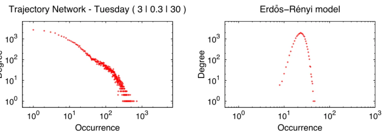
D e g re e Occurrence

Trajectory Network - Tuesday ( 3 | 0.3 | 30 )

(a)Degree distribution following a power law from a network in Chapter 4

100 101 102 103

D e g re e Occurrence

Erdõs" ïRényi model

(b) Degree distribution of a random graph gener-ated from ER model in Chapter 4 following a Pois-son distribution

Figure 3.3: Examples of degree distribution of two networks

Node Degree 1 3 2 6 3 4 4 4 5 3 6 5 7 3 (a) Degree Frequency 3 3 4 2 5 1 6 1 (b)

0 1 2 3 4 0 1 2 3 4 5 6 7 8 Frequency Degree (c)

(38)

This transitivity, also known as clustering coefficient means the presence of a number of triangles in the network, i.e., sets of three nodes each of which is connected to each of the others. There are different manners to compute clustering coefficient of a network: by finding triangles (global) or finding that coefficient for each node (local). The clustering coefficient is then defined by finding the triangles in the network as:

C = 3 x number of triangles in the network

number of connected triples of nodes , (3.1)

where a “connected triple” means a single node with edges running to an unordered pair of others. C is the mean probability for two nodes that are neighbors of the same other node are also neighbors, hence C lies in the range 0 ≤ C ≤ 1. It can also be written in the form

C = 6 x number of triangles in the network

number of paths of length two , (3.2) where a path of length two refers to a directed path starting from a specified node. Those definition of C are widely use in the sociology literature which is referred as the “fraction of transitive triples” [Newman, 2003]. On the other side, Watts and Stro-gatz [Watts & StroStro-gatz, 1998] proposed an alternative definition by defining a local value:

Ci =

number of triangles connected to node i

number of triples centered on node i . (3.3)

IntuitivelyCi of a nodeirepresents the proportion of edges between its neighbors divided

by the number of edges that there can be between them. For nodes with degree 0 or 1, their coefficient is defined asCi = 0. Thus the clustering coefficient for the whole network

is given by the average

C = 1

n

X

i

Ci. (3.4)

An interesting point about clustering coefficient refers to the fact that random graphs present low clustering coefficient when compared to real networks. So, heightened clus-tering coefficient and a large number of triangles are typical characteristics of real networks such as social network, biology networks and collaboration networks.

3.1.2.3 Shortest Path Length, Betweenness Centrality and Closeness Cen-trality

(39)

separation between two nodes in the network is given by theaverage shortest path length

L= 1

n(n−1) X

i6=j

di,j, (3.5)

wheren =|V| and di,j is the shortest path length between i and j. Random graphs and

real networks are both characterized by small average shortest path lengths, i.e., the nodes tend to reach each others, on average, in a few steps. The reachability between two nodes

i and j that are not neighbors depends on the nodes belonging to the paths connecting

i and j. A node k that belongs to many shortest paths has an important position in the network: indeed, to transfer information from a node to another, this information passes through the nodek that contributes to decrease the distances in the network and, consequently, to speed up the information propagation. This measure is known as node betweenness. Then, the betweenness of a node k is given by

bk =

X

i,j,i6=j

nij(k)

nij

, (3.6)

where nij is the number of shortest paths connecting i and j and nij(k) is the number

of shortest paths connecting iand j and passing through k. The concept of betweenness can also be used to edges, edge betweenness, which is deﬁned as the number of shortest paths pairs of node that run through that edge. As degree, the betweenness is a measure of centrality in the network, since nodes with high betweenness play an important role in decreasing the average shortest path lengths. Other measure of centrality is thecloseness centrality, which expresses the average distance of a node ito all others as

gi =

1 P

i6=jdij

. (3.7)

Therefore, the nodes with shortest distances to the other nodes will be more central in the network.

3.1.2.4 Power Law Distribution

A distribution that follows a power law is a distribution in the form

p(x) = a∗x−ω_, _(3.8)

where p(x) is the probability of x to occur, a is constant of proportionality and ω is the power law exponent [Newman, 2005]. Distributions that follow a power law are quite important for the understanding of natural and human phenomena. For instance, the population of cities and the intensity of earthquakes follow a power law distribution.

(40)

3.2 Network Models 39

Such phenomenon has also been found in real networks, i.e., degree distribution of the nodes follows a power law distribution. Such networks have many nodes with low degree, while a few nodes have high degree. Other works showed other distributions in network that also tend to follow a power law, such as the growth of the number of nodes and edges in evolving networks [Leskovec et al., 2006], and the number of triangles compared to the degree of nodes [Tsourakakis, 2008].

Although random networks and real networks present both a small average shortest path length, they are distinguished between them by their node distribution. As we have seen, degree distribution of real networks tends to follow a power law distribution. Random networks however tend to follow a Poisson distribution, i.e., the nodes tend to have the same degree. Networks with power-law degree distributions are sometimes referred to asscale-free networks [Barabási & Albert, 1999].

3.1.2.5 The Small-World Effect

The very famous experiment carried out by Stanley Milgram in the 1960s showed that letters passed from person to person were able to reach a designated target individual in only a small number of steps, sentence known as “six degrees of separation”. So, this result is one of the ﬁrst direct demonstrations of thesmall-world effect, the fact that most pairs of nodes in most networks seem to be connected by a small short path through the network.

The small-world eﬀect has implications for the dynamics of processes taking place on networks [Newman, 2003]. For instance, the spread of information across the network that occur quickly on most real networks, information like virus of computers, spam, diseases and even gossips. Networks with this behavior are characterized mainly by the two properties already discussed, i.e., they present a small average shortest path length and a high clustering coeﬃcient when compared to random networks with the same size (number of nodes and edges) [Newman, 2003].

Recently, [Backstrom et al., 2011] discovered that this average number of ac-quaintances separating any two people in the United States was 4.37, and that the number separating any two people in the world was 4.74 by using data on the links among 721 million Facebook users.

3.2 Network Models

(41)

3.2.1 Random Graphs

The study of random graphs was initiated by Erdős and Rényi in 1959 with the original purpose of studying, by means of probabilistic methods, the properties of graphs as a function of the increasing number of random connections. Erdős and Rényi proposed a model to generate random graph with n nodes and m edges, which is known as ER random graphs [Erdős & Rényi, 1959, Erdős & Rényi, 1960]. There are two diﬀerent ways to construct a network from this model:

• Gn,p is a random graph generated by taking some number n of nodes and connect

each pair with probability p;

• Gn,m is the ensemble of all graphs havingn nodes and exactlymedges, each possible

graph appearing with equal probability.

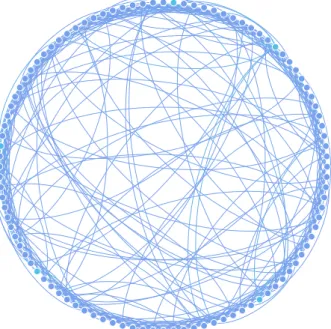
ER random graphs are the most studied among graph models, although they do not reproduce most of the properties of real networks, such as clustering coeﬃcient. A small average shortest path length characterizes the random graphs, even though they do not present many triangles as we discussed early. In addition, random graphs present a Poisson distribution, while real networks tend to follow a power law distribution. Fig-ure 3.5 depicts a random graphGn,p with n = 50 and p= 0.05.

Figure 3.5: A random graph Gn,p generated with n = 100 and p = 0.05. Its average

(42)

Figure 3.6: The small world model varying p. This ﬁgure illustrates well the network structure by varying the probability p: p = 0 generates a regular network, while p = 1

generates a random network [Watts & Strogatz, 1998]

3.2.2 Small-World Model

Watts and Strogatz proposed a model, known as small-world or WS model, to study and identify properties of small-world effect, i.e., a high transitivity and a small average shortest path length [Watts & Strogatz, 1998]. The small-world model starts withnnodes shaping a ring where each node is connected to itsk nearest neighbors, that is,k/2on its left side andk/2on its right side. This ﬁrst process generates a regular lattice. Forthwith, a process of “rewiring” is achieved, where each edge has its one end moved, with probability

p, to a new location chosen uniformly at random from the lattice, except that no double edges or self-edges are ever created.

The rewiring process allows the small-world model to interpolate between a regular lattice and something similar to random graph. When p = 0, the generated network will be a regular lattice. However, the regular lattice does not show the small-world eﬀect, since the path lengths tend to be large from a node to another. Whenp= 1, every edge is rewired to a new random location and the network looks like a random graph, with a small average shortest path, but with very low clustering coeﬃcient. Therefore,p

works as a balancer between regular lattice and something random as showed in Figure 3.6. A generated network from this small-world model is illustrated in Figure 3.7

Due to the simplicity of the original model proposed by Watts and Strogatz, where only one end of each chosen edge is rewired, no node is ever connected to itself and an edge is never added between node pairs where there is already one, many other small-world models were proposed [Monasson, 1999, Newman & Watts, 1999].

3.2.3 Models of Network Growth

(43)

Figure 3.7: A WS network shaping a ring generated with n = 100 and p = 0.2 and

k = 10. Its average shortest path is 2.548 and its clustering coeﬃcient is 0.419 (624 triangles)

understanding how networks come to have such properties. In other words, they do not take into consideration the process of growth of networks and, hence, they are not models of network growth. From this, Barabási and Albert proposed the model known as Barabási-Albert (BA) orPreferential Attachment model [Barabási & Albert, 1999], which is based on two aspects: growth and preferential attachment.

The main idea of BA model goes towards the phenomenon “the rich get richer”. Speaking in network terms, the nodes with highest degrees (“the rich”) are likely to form new edges with other nodes (“get richer”), and those nodes are called preferential attach-ment. More precisely, an undirected graph Gn,k is constructed from BA model as follows.

Starting with m0 isolated nodes, at each time step t = 1,2,3, . . . , N −m0 a new node j withm≤m0 links is added to the network. Then, the probability that a link will connect

j to an existing nodeiis linearly proportional to the degree of i. Despite of being elegant and simple, BA model lacks some features that are present in the real World Wide Web, such as the directness of the edges. Figure 3.8 shows an example ofGn,k.

(44)

3.3 Community Discovery 43

Figure 3.8: A BA network generated with n= 100 and m0 = 4and k= 2. The largest and red nodes represent the preferential attachments, highly connected nodes, which are more likely to establish new links with other nodes

3.3 Community Discovery

As we have discussed so far, many properties are computer over nodes and edges to catch global or local behaviors of the network. However, another important part of the network research is related to the network structure, that is, how the nodes connect to each other forming groups together called communities. Take as example people that form groups with other people in diﬀerent contexts, such as our friends from work, university and even gym. Each context may correspond, somehow, to communities of a network of people.

According to [Newman, 2003], community discovery should not be confused with the technique of data clustering, which is a way of detecting groupings of data-points in high-dimensional data spaces. Community discovery and data clustering have some common features and algorithms for one can be adapted to the other, and vice-versa. For example, high-dimensional data can be converted into a network by placing edges between closely spaced data points, and then network clustering algorithms can be applied to the result. On balance, however, one normally ﬁnds that algorithms specially devised for data clustering work better than such borrowed methods, and the same is true in reverse.

(45)

3.3 Community Discovery 44

Figure 3.9: An example of community discovery by perfoming the method proposed in [Blondel et al., 2008]. This algorithm is available in Gephi [Bastian et al., 2009]. This network was built from a user’s proﬁle in a social network and, thus, each community represented by a color shows a community of people. For instance, the blue community represents the friends from the university and the red one represents the family ties

community detection does not have a unique concept or deﬁnition. As consequence, a broad variety of methods have been proposed to discovery communities.

In front of these great variety of techniques, [Coscia et al., 2011] proposed a classiﬁcation for community discovery methods in complex networks. Some methods take nodes as entities, that is, nodes are compared to each other to compute their similarity, while others consider edges as entities in order to group the edges and further the nodes. In addition, there are a number of interesting features of these communities that can be considered, such as hierarchical or overlapping conﬁguration of the groups inside the network, the directness of the edges to give importance to this direction when considering the relations among entities and, yet, the dynamism of the networks, i.e., networks that evolve over time.

(46)

3.4 Summary 45

3.4 Summary

This chapter introduced basic concepts and deﬁnitions in complex networks, presenting some important deﬁnitions in graph theory, which is the basis of networks. In addition, this chapter presented some global and local properties of networks that are important not only for understanding of network topologies, but also for comprehension of network behaviors.

Some network models present in the literature were discussed, including the ER model proposed by [Erdős & Rényi, 1959, Erdős & Rényi, 1960], the WS model proposed by [Watts & Strogatz, 1998] to capture the behavior of networks with small-world eﬀects, and the Preferential Attachment model proposed by [Barabási & Albert, 1999] in order to understand the growth of networks based on preferential attachment.

(47)

4 Trajectory Analysis using Complex Network 46

CHAPTER

4

Trajectory Analysis using Complex

Network

A

lthough the management of trajectory data dates back to the 1990s, when the first proposals for moving object databases came out, the challenging approaches towards the analysis and understanding of the movement complexity represented in the users tracks is being faced only recently [Wang et al., 2009]. Even more challenging is the aspect of moving object interaction. How and how much do these moving objects interact? How do theencountersamong moving entities globally characterize the movement of a moving community? Is there a specific law explaining the interactions of moving individuals? Is the movement of people in vehicles (e.g. cars in a road network) differs from people free movement and/or multi transportation trajectories? How do the individual movements of independent entities influence a crowd’s movement pattern?

(48)

4.1 Basic Concepts and Related Work 47

networks experiments, which focuses on objects that are “static”, from the point of view of the spatial position.

The contributions present in this chapter are twofold. The first contribution is a method for devising a complex network from a trajectory dataset, hereinafter called trajectory network. The aim of this method is to define specific steps for processing trajectory data in order to build and analyze the trajectory network. The second contri-bution is an algorithm for building a trajectory network given a trajectory dataset (set of spatio-temporal points). Indeed, this is the first work on analyzing trajectory interactions through complex network techniques [Brilhante et al., 2011].

The proposed method has been evaluated using a real GPS dataset from ve-hicles moving in the City of Milan. All generated trajectory networks from this dataset presented the small world eﬀect and the scale-free feature similar to the Internet and bio-logical networks. However the interpretation of these features is an open issue, therefore we will discuss possible interpretations and exploitations of them.

This chapter is structured as follows. Section 4.1 reviews some basic deﬁnitions introduced in Chapter 2 and 3, and introduces related works. Section 4.2 presents the methods and algorithms used to build the trajectory complex network, whereas Section 4.3 reports experimental results carried on a complex network of vehicle trajectories. Section 4.4 draws conclusions and future work.

4.1 Basic Concepts and Related Work

4.1.1 Basic Definitions

As presented in Chapter 2, a trajectory can be deﬁned as the spatio-temporal evolution of a moving object [Spaccapietra et al., 2008]. This evolution is typically represented as a sequence of sample points, representing the spatio-temporal positions detected by a tracking device, such as GPS tools or WIFI sensors. More formally, a trajectory T of an object O is represented as: TO= {p0, p1, ..., pn}, where pi = (xi, yi, ti), xi, yi ∈ R

represent the spatial coordinates of the sample point ,ti ∈R+ represents the timestamp

fori= 0,1, ..., n, and t0< t1< t2< . . . < tn.

In Chapter 3, acomplex networkis introduced as a network with thousands or

millions of nodes whose structure is irregular, with non-trivial topology features [Boccaletti et al., 2006]. The following features typically characterize complex networks:

• Clustering coefficient: represents the density of triangles in the network. Sparse ran-dom graphs have smaller clustering coefficients, while real-world networks typically have larger coefficients;

(49)

4.1 Basic Concepts and Related Work 48

• Power law distribution: is a distribution that follows a power law function, p(x) =

a ∗ x−α_{, such that} _p₍_x₎ _{is the probability of occurrence of x,} _a _{is a constant of}

proportionality and α is the power law exponent.

Complex networks can be characterized by the so called “small world” prop-erty when the average number of edges between any two vertices is very small and the clustering coeﬃcient is large [Watts & Strogatz, 1998]. Intuitively, this represents a short path between two edges. This is also known as the “six degrees of separation”. Scale free networks are characterized by a degree distribution that follows a power law func-tion. Intuitively, few nodes have many edges (the “hubs” or preferential attachment [Barabási & Albert, 1999] ), many nodes have few edges.

4.1.2 Mobility Analysis

With the increasing availabilities of trajectory datasets collected from GSM or GPS equipped devices we have the possibility of studying people behavior from their move-ment traces. Several application areas would beneﬁt from an extensive study on people trajectories such as traﬃc management, public transportation, commercial advertising, security and police, hazard evacuation management, location based services and so on.

The task of analyzing large trajectory datasets can be carried out in four diﬀer-ent directions. First, basic statistics may be applied to trajectory data mainly to discover the distributions of people presence and origin-destination matrices [Calabrese et al., 2010]; other studies focus on trajectory data mining, that is, on the application of data min-ing techniques to trajectory data [Giannotti & Pedreschi, 2008]; other researches focus on representing and querying moving objects in database systems [Nguyen-Dinh et al., 2010, Güting et al., 2000]; ﬁnally, research originally coming from Physics studies mathemati-cal models, such as complex networks, representing the general laws that describe human movement [González et al., 2008, Wang et al., 2009].

Trajectory mining aims at finding correlations in large datasets of trajectory data, collected by personal positioning devices. Techniques include: (1) clustering discovery finding groups of objects moving together; (2) sequential pattern disdiscovery -finding the most frequent sequences of places visited; (3) flock detection - extracting the convergence of people moving together for a certain amount of time [Dodge et al., 2008, Giannotti & Pedreschi, 2008].

Several works have investigated how to model and query movement data ef-ﬁciently, in database literature a new class of databaase systems were created, called moving object database [Nguyen-Dinh et al., 2010, Güting et al., 2000]. However, these works were not focused in modeling or querying trajectory data as a ﬁrst class object. In addition, they did not aim at exploring moving objects interactions.

(50)

4.2 Complex Network and Trajectory 49

study the physical laws representing human movements. Social interactions is also in the scope of this research area. A typical example is the study of the spreading of cell phone viruses thru GSM phone calls [Wang et al., 2009].

4.1.3 Complex Network Analysis

As already presented in the previous section and Chapter 2, a network is a set of items, called vertices (or nodes), with connections among them, called edges (or links). The study of networks (in the form of mathematical graph theory) is one the fundamental pillars of discrete mathematics. Networks have also been extensively studied in diﬀerent domains, such as Social sciences, Physics, etc. However, recent years have witnessed a substantial new movement in network research, focusing on developing methods and techniques to gather and analyze networks far larger than previously possible. Indeed, this new motivation is due to the inability of humans to draw a meaningful picture of a million vertices by direct eye analysis.

Network has been used as a mechanism of analyses of a huge amount of data with a set of objects which have a relationship or a interaction between them. For in-stance, the studies in psychology where a node represents a person and an edge represents friendship or that they work together or simply that they know each other or even they have sexual relationship; the studies in biology where the focus is on the species in an ecosystem and a interaction between them, that is, an edge (directed) from species A to species B indicates that A preys B [Pimm, 2002]. Therefore, networks oﬀer a perspective of analyses basing on the relationships or interactions.

With respect to mobility analysis, [Guo et al., 2010] presents a graph-based approach to represent the trajectories by using representative points, a new set of points based on the original one, to generate a graph and find clusters of trajectories. However, they do not consider the properties of the complex network area such as clustering co-efficient. On other hand, [Kaluza et al., 2010] analyzes global cargo ship movements by building a complex network whose nodes represent the ports and links represent the ship traffic between two ports. Differently from our approach, they do not represent the nodes as trajectories and, besides, the points of the trajectories are not taken into account, but only the ports that the cargo ships passed.

4.2 Complex Network and Trajectory

This section presents one approach about how to create a complex network from trajectory data. This approach constructs a simple graph where each node represents a trajectory and each edge represents a relationship among the nodes. A relationship between two nodes is established when there is an encounter between two trajectories in space and time with a minimum frequency of meetings.

(51)

4.2 Complex Network and Trajectory 50

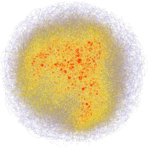
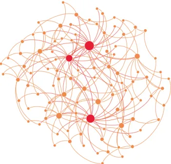
Figure 4.1: A plotted complex network composed by 36,824 nodes and 306,572 edges generated in our experiments

the help of a similarity function f between trajectories in S and a threshold constant

c. This network is called trajectory network. The trajectory network (N,E) is constructed as follows: (1) each node in N represents a trajectory in S; (2) there is an edge between two nodesn and m iﬀ f(m, n)≥c, that is,m and n represent trajectories whose similarity is above the given threshold.

In what follows, we will not distinguish between trajectories inS and nodes in

N.

We therefore deﬁne a functionf to capture the spatial and temporal proximity between two trajectories in order to establish an edge between them in the network. Let

f be the similarity function for trajectories used to construct the trajectory network, and lets,t and k respectively be the spatial, temporal and frequency parameters of f. Given a trajectoryT, the spatial and temporal parameters induce a buﬀer B[s, t](T) aroundT. Given two trajectories T and U, we then deﬁne:

Definition 4.1 meet (or collide): T and U meet iff B[s, t](T) and B[s, t](U) overlap.

Mobility Data under Analysis a Complex Network Perspective from Interactions Among Trajectories to Movements among Points Interest

Universidade Federal do Ceará

Departamento de Computação

Curso de Ciência da Computação

Igo Ramalho Brilhante

Mobility data analysis under a complex network perspective:

from interactions among trajectories to movements among points

of interest

Igo Ramalho Brilhante

Mobility data analysis under a complex network perspective:

from interactions among trajectories to movements among points

of interest

Abstract

List of Figures

List of Tables

List of Algorithms

Contents

CHAPTER

1

Introduction

T

1.1

Motivation

1.2

Contributions

1.3

Publications

1.4

Organization

CHAPTER

2

Mobility Analysis

T

2.1

Preliminaries

2.1.1

Trajectory

2.1.2

Semantic Trajectory

2.2

Stops and Moves

2.3

Identifying Stops and Moves

2.3.1

SMoT (Stops and Moves of Trajectories)

2.3.2

CB-SMoT (Clustering-Based SMoT)

2.3.3

Stay Point Detection

2.4

Summary

CHAPTER

3

Complex Network

R

3.1

Preliminaries

3.1.1

Concepts and Basic Definitions

3.1.2

Properties of Complex Networks

3.2

Network Models

3.2.1

Random Graphs

3.2.2

Small-World Model

3.2.3

Models of Network Growth

3.3

Community Discovery

3.4

Summary

CHAPTER

4

Trajectory Analysis using Complex

Network

A

4.1

Basic Concepts and Related Work