Aerosol indirect effects in a multi-scale aerosol-climate model PNNL-MMF

(1)

ACPD

11, 3399–3459, 2011

Indirect e_ffects in an aerosol-climate model PNNL-MMF

M. Wang et al.

Title Page

Abstract Introduction

Conclusions References

Tables Figures

◭ ◮

Back Close

Full Screen / Esc

Printer-friendly Version

Interactive Discussion

Discussion

P

a

per

|

Dis

cussion

P

a

per

|

Discussion

P

a

per

|

Discussio

n

P

a

per

Atmos. Chem. Phys. Discuss., 11, 3399–3459, 2011 www.atmos-chem-phys-discuss.net/11/3399/2011/ doi:10.5194/acpd-11-3399-2011

Atmospheric Chemistry and Physics Discussions

This discussion paper is/has been under review for the journal Atmospheric Chemistry and Physics (ACP). Please refer to the corresponding final paper in ACP if available.

Aerosol indirect e

_ff

ects in a multi-scale

aerosol-climate model PNNL-MMF

M. Wang1, S. Ghan1, M. Ovchinnikov1, X. Liu1, R. Easter1, E. Kassianov1, Y. Qian1, and H. Morrison2

1

Atmospheric Science and Global Change Division, Pacific Northwest National Laboratory, Richland, Washington, USA

2

Mesoscale and Microscale Meteorology Division, National Center for Atmospheric Research, Boulder, Colorado, USA

Received: 14 January 2011 – Accepted: 19 January 2011 – Published: 31 January 2011 Correspondence to: M. Wang (minghuai.wang@pnl.gov)

(2)

ACPD

11, 3399–3459, 2011

M. Wang et al.

Title Page

Tables Figures

◭ ◮

Back Close

Full Screen / Esc

Discussion

P

a

per

|

Dis

cussion

P

a

per

|

Discussion

P

a

per

|

Discussio

n

P

a

per

|

Abstract

Much of the large uncertainty in estimates of anthropogenic aerosol e_ffects on cli-mate arises from the multi-scale nature of the interactions between aerosols, clouds and large-scale dynamics, which are difficult to represent in conventional global cli-mate models (GCMs). In this study, we use a multi-scale aerosol-clicli-mate model that 5

treats aerosols and clouds across multiple scales to study aerosol indirect effects. This multi-scale aerosol-climate model is an extension of a multi-scale modeling framework (MMF) model that embeds a cloud-resolving model (CRM) within each grid cell of a GCM. The extension allows the explicit simulation of aerosol/cloud interactions in both stratiform and convective clouds on the global scale in a computationally feasible 10

way. Simulated model fields, including liquid water path (LWP), ice water path, cloud fraction, shortwave and longwave cloud forcing, precipitation, water vapor, and cloud droplet number concentration are in agreement with observations. The new model performs quantitatively similar to the previous version of the MMF model in terms of simulated cloud fraction and precipitation. The simulated change in shortwave cloud 15

forcing from anthropogenic aerosols is−0.77 W m−2, which is less than half of that in

the host GCM (NCAR CAM5) (−1.79 W m−2) and is also at the low end of the estimates

of most other conventional global aerosol-climate models. The smaller forcing in the MMF model is attributed to its smaller increase in LWP from preindustrial conditions (PI) to present day (PD): 3.9% in the MMF, compared with 15.6% increase in LWP in 20

large-scale clouds in CAM5. The much smaller increase in LWP in the MMF is caused by a much smaller response in LWP to a given perturbation in cloud condensation nu-clei (CCN) concentrations from PI to PD in the MMF (about one-third of that in CAM5), and, to a lesser extent, by a smaller relative increase in CCN concentrations from PI to PD in the MMF (about 26% smaller than that in CAM5). The smaller relative increase 25

(3)

ACPD

11, 3399–3459, 2011

M. Wang et al.

Title Page

Tables Figures

◭ ◮

Back Close

Full Screen / Esc

Discussion

P

a

per

|

Dis

cussion

P

a

per

|

Discussion

P

a

per

|

Discussio

n

P

a

per

the MMF model is consistent with observations and with high resolution model studies, which may indicate that aerosol indirect effects simulated in conventional global climate models are overestimated and point to the need to use global high resolution models, such as MMF models or global CRMs, to study aerosol indirect effects. The simulated total anthropogenic aerosol effect in the MMF is −1.05 W m−2, which is close to the 5

Murphy et al. (2009) inverse estimate of₋1.1_±0.4 W m−2₍₁_σ_{) based on the}

examina-tion of the Earth’s energy balance. Further improvements in the representaexamina-tion of ice nucleation and low clouds are needed.

1 Introduction

Clouds are an extremely important climate regulator. They have a large impact on 10

the Earth’s energy budget and play a central role in the hydrological cycle. By acting as cloud condensation nuclei (CCN) or ice nuclei, anthropogenic aerosols can modify cloud optical and physical properties, and therefore affect the climate system, giving rise to the so-called the aerosol indirect effect. Uncertainties in estimates of the anthro-pogenic aerosol indirect e_ffect still dominate uncertainties in the estimates of radiative 15

forcing of past and future climate change, despite more than a decade of effort on this issue (Forster et al., 2007; IPCC, 2007; Lohmann et al., 2010).

Much of this uncertainty arises from the multi-scale nature of the interactions be-tween aerosol, clouds, and large-scale dynamics. These interactions span a wide range in spatial scales, from 0.01–10 µm for droplet and crystal nucleation, to 10– 20

1000 m for turbulence-driven updrafts, to 2–10 km for deep convection, to 50–100 km for large-scale cloud systems. Given the typical global climate model (GCM) grid spac-ing of a hundred kilometers, the treatment of most of those processes is highly param-eterized in conventional GCMs and therefore may not be accurate.

One example is cloud lifetime effects of aerosol. As implemented in most GCMs, 25

(4)

ACPD

11, 3399–3459, 2011

M. Wang et al.

Title Page

Tables Figures

◭ ◮

Back Close

Full Screen / Esc

Discussion

P

a

per

|

Dis

cussion

P

a

per

|

Discussion

P

a

per

|

Discussio

n

P

a

per

|

anthropogenic aerosols always slows formation of precipitation and increases liquid water path (LWP) and cloud lifetime (Albrecht, 1989). However, observations show evidence of both decreasing and increasing LWP with increasing aerosols (Platnick et al., 2000; Coakley and Walsh, 2002; Kaufman et al., 2005; Matsui et al., 2006), and cloud resolving model (CRM) studies show that whether LWP increases or decreases 5

with increasing aerosols depends on meteorological conditions (Ackerman et al., 2004; Xue et al., 2008; Small et al., 2009).

It is even more problematic to represent aerosol/cloud processes in deep cumulus clouds in GCMs. Cumulus parameterizations in current climate models rely on ad hoc closure assumptions designed to diagnose the latent heating and vertical transport 10

of heat and moisture by deep convection, and provide little information about micro-physics or updraft velocity (Emanuel and Zivkovic-Rothman, 1999; Del Genio et al., 2005; Zhang et al., 2005). As a result, only a handful of GCMs have treated aerosol e_ffects on convective clouds in their estimates of aerosol indirect e_ffects (Menon and Rotstayn, 2006; Lohmann, 2008), and because those treatments were based on con-15

ventional cumulus parameterizations, the treatments are quite crude. Menon and Rot-stayn (2006) introduced a physically-based treatment of aerosol effects on convective cloud microphysics in two GCMs and found a strong dependence of indirect e_ffects on the details of the cumulus parameterization: including aerosol effects on convective clouds increased aerosol indirect effects in one GCM but slightly decreased aerosol 20

indirect e_ffects in the other GCM. Lohmann (2008) investigated aerosol e_ffects on con-vective clouds by extending a double-moment cloud microphysics scheme developed for stratiform clouds to convective clouds, and found that including aerosol effects in convective clouds reduces the sensitivity of the LWP to aerosol optical depth (AOD), which is in better agreement with observations and large-eddy simulation studies and 25

(5)

ACPD

11, 3399–3459, 2011

M. Wang et al.

Title Page

Tables Figures

◭ ◮

Back Close

Full Screen / Esc

Discussion

P

a

per

|

Dis

cussion

P

a

per

|

Discussion

P

a

per

|

Discussio

n

P

a

per

We have recently developed a multi-scale aerosol-climate model (Wang et al., 2010), which is an extension of a multi-scale modeling framework (MMF) model that embeds a CRM within each grid column of a GCM (Khairoutdinov et al., 2008). The GCM compo-nent includes a modal aerosol treatment that uses several log-normal modes to repre-sent aerosol size distributions. The CRM component has a two-moment microphysics 5

scheme and predicts both mass and number mixing ratios for all hydrometeor types. Cloud statistics diagnosed from the CRM component are used to drive the aerosol and trace gas processing by clouds. This multi-scale aerosol-climate model allows us to explicitly simulate aerosol/cloud interactions in both stratiform and convective clouds. Compared to global CRMs with on-line aerosols (Suzuki et al., 2008), this multi-scale 10

aerosol-climate model is computationally much more feasible for running multi-year climate simulations. Wang et al. (2010) showed that this multi-scale aerosol-climate model simulates aerosol fields as well as conventional aerosol-climate models.

In this study, we evaluate simulated cloud fields from this multi-scale aerosol-climate model, and examine anthropogenic aerosol e_ffects on clouds and climate. Section 2 15

describes the model. Model results with the present day aerosol and precursor emis-sions are shown in Sect. 3. The aerosol indirect effects are examined in Sect. 4 and finally the results are summarized in Sect. 5.

2 Model description and set-up of simulations

2.1 Model description

20

The PNNL-MMF is documented in detail in Wang et al. (2010) and is only briefly de-scribed here. It is an extension of the Colorado State University (CSU) MMF model (Randall et al., 2003; Khairoutdinov et al., 2005, 2008; Tao et al., 2009), first developed by Khairoutdinov and Randall (2001). The host GCM in the PNNL-MMF is the Commu-nity Atmospheric Model version 5 (CAM5) (http://www.cesm.ucar.edu/models/cesm1. 25

(6)

ACPD

11, 3399–3459, 2011

M. Wang et al.

Title Page

Tables Figures

◭ ◮

Back Close

Full Screen / Esc

Discussion

P

a

per

|

Dis

cussion

P

a

per

|

Discussion

P

a

per

|

Discussio

n

P

a

per

|

(CESM1.0). The embedded CRM in each GCM grid column is a two-dimensional version of the System for Atmospheric Modeling (SAM) (Khairoutdinov and Randall, 2003), which replaces the conventional moist physics, convective cloud, turbulence, and boundary layer parameterizations in CAM5. During each GCM time step (every 10 min), the CRM is forced by the large-scale temperature and moisture tendencies 5

arising from GCM-scale dynamical processes and feeds the cloud response back to the GCM-scale as heating and moistening terms in the large-scale budget equations for heat and moisture. The CRM runs continuously using a 20-s time step.

The version of the SAM CRM used in this study features a two-moment cloud crophysics scheme (Morrison et al., 2005, 2009), which replaces the simple bulk mi-10

crophysics used in the original CSU MMF model. The new scheme predicts the num-ber concentrations and mass mixing ratios of five hydrometeor types (cloud droplets, ice crystals, rain droplets, snow particles, and graupel particles). The precipitation hydrometeor types (rain, snow, and graupel) are fully prognostic in the CRM model, rather than diagnostic in CAM5 (Morrison and Gettelman, 2008). Droplet activation 15

from hydrophilic aerosols, ice nucleation, ice crystal growth by vapor deposition, the dependence of ice crystal sedimentation on crystal number, and the dependence of autoconversion on droplet number are treated. Several ice nucleation mecha-nisms are included: contact nucleation of cloud droplets following Morrison and Pinto (2005); immersion freezing of cloud droplets and rain following Bigg (1953); deposition-20

condensation freezing nucleation following Thompson et al. (2004), which is based on ice crystal concentration measurements of Cooper (1986) and limited to a maximum of 0.5 cm−3_{; and homogenous freezing of all cloud and rain drops below}

−40◦C. These

ice nucleation treatments do not directly link heterogeneous ice nuclei to aerosols. Droplet activation is calculated at each CRM grid cell, based on the parameterization 25

(7)

ACPD

11, 3399–3459, 2011

M. Wang et al.

Title Page

Tables Figures

◭ ◮

Back Close

Full Screen / Esc

Discussion

P

a

per

|

Dis

cussion

P

a

per

|

Discussion

P

a

per

|

Discussio

n

P

a

per

CAM5, the driving GCM, uses a modal approach to treat aerosols (Liu et al., 2011) on the CAM5 grid. Aerosol size distributions are represented by using three log-normal modes: an Aitken mode, an accumulation mode, and a single coarse mode. Aitken mode species include sulfate, secondary organic aerosol (SOA), and sea salt; ac-cumulation mode species include sulfate, SOA, black carbon (BC), primary organic 5

matter (POM), sea salt, and dust; coarse mode species include sea salt, dust, and sul-fate. Species mass and number mixing ratios are predicted for each mode, while mode widths are prescribed. Aerosols outside cloud droplets (interstitial) and aerosols within cloud droplets (cloud-borne) are both predicted. Aerosol nucleation (involving H₂SO₄ vapor), condensation of trace gases (H₂SO₄ and semi-volatile organics) on existing 10

aerosol particles, and coagulation (Aitken and accumulation modes) are also treated. In the PNNL MMF, the treatment of cloud-related aerosol and trace gas processes (i.e., aqueous chemistry, convective transport, and wet scavenging) in the stan-dard CAM5 is replaced by the explicit-cloud-parameterized-pollutant (ECPP) approach (Gustafson et al., 2008; Wang et al., 2010). The ECPP approach uses statistics of 15

cloud distribution, vertical velocity, and cloud microphysical properties resolved by the CRM to drive aerosol and chemical processing by clouds on the GCM grid, which allows us to explicitly treat the e_ffects of convective clouds on aerosols in computa-tionally feasible manner. The ECPP approach predicts both interstitial aerosols and borne aerosols in all clouds, while the conventional CAM5 only treats cloud-20

borne aerosols in stratiform clouds. In addition, by integrating the continuity equation for aerosols and trace gases in convective updraft and downdraft regions, the ECPP approach treats convective transport, aqueous chemistry, and wet scavenging in an integrated, self-consistent way (Wang et al., 2010).

The CAM5 radiative transfer scheme uses the Rapid Radiative Transfer Model for 25

(8)

ACPD

11, 3399–3459, 2011

M. Wang et al.

Title Page

Tables Figures

◭ ◮

Back Close

Full Screen / Esc

Discussion

P

a

per

|

Dis

cussion

P

a

per

|

Discussion

P

a

per

|

Discussio

n

P

a

per

|

on the CRM grid from the dry aerosol on the GCM grid, and the aerosol water on the CRM grid that is calculated from Kohler theory based on the relative humidity on the CRM grid, accounting for hysteresis and the hygroscopicities of each of the modes’ components (Ghan and Zaveri, 2007).

2.2 Emissions and set-up of simulations

5

The host GCM CAM5 uses a finite-volume dynamical core, with 30 vertical levels at 1.9◦×2.5◦ horizontal resolution. The GCM time step is 10 min. Climatological

sea surface temperature and sea ice are prescribed. The embedded CRM includes 32 columns at 4-km horizontal grid spacing and 28 vertical layers coinciding with the lowest 28 CAM levels. The time step for the embedded CRM is 20 s. The MMF model 10

was integrated for 36 months. Results from the last 34 months are used in this study. Results from the MMF model are also compared with those from the conventional CAM5. The conventional CAM5 runs at 1.9◦×2.5◦ horizontal resolution with 30

verti-cal levels and a time step of 30 min, and was integrated for 5 years. Results from the last four years are reported here. The three-mode aerosol scheme and the modified 15

Morrison-Gettelman two-moment cloud scheme are used for large-scale processes in CAM5 (Gettelman et al., 2010), and shallow and deep convective clouds are parame-terized with no explicit aerosol e_ffects.

Both the MMF and CAM5 use the same aerosol and precursor emissions as de-scribed in Liu et al. (2011) and Wang et al. (2010). Anthropogenic SO₂, BC, and 20

primary organic carbon emissions are from the Lamarque et al. (2010) IPCC AR5 emission data set. The years 2000 and 1850 are chosen to represent the present day (PD) and the pre-industrial (PI) time, respectively. Volcanic SO₂ and DMS emissions are taken from Dentener et al. (2006), and 2.5% of SO₂emissions are emitted as pri-mary sulfate aerosol. Aerosol number emissions are derived from mass emissions us-25

(9)

ACPD

11, 3399–3459, 2011

M. Wang et al.

Title Page

Tables Figures

◭ ◮

Back Close

Full Screen / Esc

Discussion

P

a

per

|

Dis

cussion

P

a

per

|

Discussion

P

a

per

|

Discussio

n

P

a

per

primary volatile organic compound (VOC) classes (Liu et al., 2011), rather than being formed by atmospheric oxidation. The VOC emissions are taken from the MOZART-2 data set (Horowitz et al., 2003). Gas-phase SOA (g) partitions to the aerosol phase to form SOA aerosol through the thermodynamical transfer process. Emissions of sea salt and mineral dust aerosols are calculated online. The sea salt emissions parameteriza-5

tion follows Martensson et al. (2003) and particles with diameters between 0.02–0.08, 0.08–1.0, and 1.0–10.0 µm are placed in the Aitken, accumulation, and coarse modes, respectively. Mineral dust emissions are calculated with the Dust Entrainment and De-position Model (Zender et al., 2003); the implementation in CAM has been described in Mahowald et al. (2006a, b) and Yoshioka et al. (2007). Dust particles with diameters 10

between 0.1–1.0 and 1.0–10.0 µm are placed in the accumulation and coarse modes, respectively.

Two simulations are performed for both the MMF and CAM5: one with the PD aerosol and precursor emissions, and the other with the PI aerosol and precursor emissions. Greenhouse gases are fixed at the present day level in all simulations.

15

3 Model results in the PD simulations

3.1 Cloud fields

3.1.1 Global and annual averages

Table 1 lists global annual means of simulated cloud and radiation parameters in the MMF, along with those from the conventional CAM5 and observations. The liquid wa-20

ter path (LWP) in the MMF simulation is 55.9 g m−2_{, which is slightly larger than the}

(10)

ACPD

11, 3399–3459, 2011

M. Wang et al.

Title Page

Tables Figures

◭ ◮

Back Close

Full Screen / Esc

Discussion

P

a

per

|

Dis

cussion

P

a

per

|

Discussion

P

a

per

|

Discussio

n

P

a

per

|

in CAM5 (121 cm−3_{). Cloud-top droplet e}

ffective radius in the MMF is 9.2 µm, which is slightly smaller than that in CAM5 (9.7 µm), and both underestimate observations (11.4–15.7 µm). Simulated column-integrated grid-mean cloud droplet number con-centration (2.3_×1010 m−2_{) is nearly 50% higher than that in CAM5 (1.6}

×1010m−2).

The large difference in column-integrated cloud droplet number concentrations be-5

tween the MMF and CAM5 can be partly explained by the fact that column-integrated cloud droplet number concentration in CAM5 only includes contributions from large-scale clouds while the MMF includes contributions from both large-large-scale and convec-tive clouds.

Simulated cloud ice water path, snow water path, and graupel water path are 9.9, 10

53.4, and 5.7 g m−2, respectively. The total frozen water path is 69.0 g m−2and is close to that simulated in CAM5 (61.3 g m−2_{). It is also close to that retrieved from}

Cloud-Sat (around 80 g m−2_{), and MODIS (60 g m}−2_{), but is much larger than estimates from}

ISCCP (around 35 g m−2) and NOAA NESDIS (around 10 g m−2) (Fig. 18 in Waliser et al., 2009). CloudSat retrievals are sensitive to large hydrometeor particles and are 15

considered to be more representative of total frozen water (Waliser et al., 2009). The partitioning of total frozen water among different ice hydrometeor components is similar to that in the NASA fvMMF model (Waliser et al., 2009), which is another MMF model treating multiple hydrometeor types (Tao et al., 2009). Both the PNNL MMF and NASA fvMMF simulate a small contribution from cloud ice water over the tropics (30◦S–30◦N) 20

(13% in the PNNL MMF, compared with 10% in the NASA fvMMF). However, the PNNL MMF produces a much smaller contribution from graupel (14%), compared with that in the NASA fvMMF (50%). These differences may result from the differences in the microphysics schemes in the CRM components in the two MMF models. Given the fact that no global observation is able to distinguish di_fferent ice hydrometeors, it is still 25

difficult to constrain the partitioning among different hydrometeors in GCMs.

Simulated column-integrated ice crystal number concentration is 0.021×1010m−2,

(11)

ACPD

11, 3399–3459, 2011

M. Wang et al.

Title Page

Tables Figures

◭ ◮

Back Close

Full Screen / Esc

Discussion

P

a

per

|

Dis

cussion

P

a

per

|

Discussion

P

a

per

|

Discussio

n

P

a

per

ice crystal number concentration through the freezing of cloud droplets activated on aerosols. In CAM5, sulfate can form ice crystals in cirrus clouds through homoge-neous freezing, and dust can act as heterogehomoge-neous ice nuclei in cirrus and mixed-phase clouds (Gettelman et al., 2010). Large uncertainties exist in simulated column-integrated ice crystal number concentrations in global climate models (ranges 0.1– 5

0.7_×1010m−2 _{in Lohmann et al. (2008); 0.02–0.09}

×1010m−2 in Wang and Penner,

2010). Heterogeneous nucleation in cirrus clouds generally leads to lower column-integrated ice crystal number concentrations in better agreement with observed ice crystal number concentrations in the upper troposphere (Wang and Penner, 2010). Aerosol effects on ice nucleation in the MMF will be the subject of a future study. 10

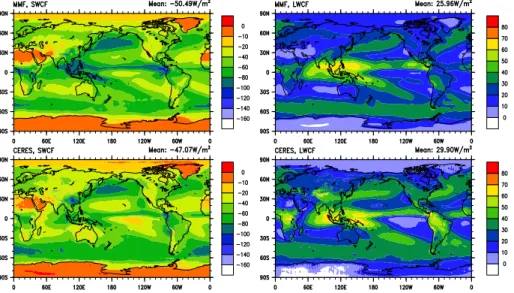
The total cloud fraction is 55.8%, which is smaller than that in CAM5 (62.7%) and in observations (65–75%). Simulated high cloud fraction, 29.2%, is smaller than that in CAM5. Shortwave cloud forcing is−50.5 W m−2, which is in the observed range (−47

to−54 W m−2) and is close to that in CAM5 (−50 W m−2). Simulated longwave cloud

forcing is 26 W m−2_{, slightly smaller than ERBE (30 W m}−2_{) and CERES (29 W m}−2₎ 15

observations, and is larger than that simulated in CAM5 (22 W m−2). Simulated precip-itation rate is 2.85 mm day−1_{, higher than observations (2.61 mm day}−1_).

3.1.2 Global and zonal distributions

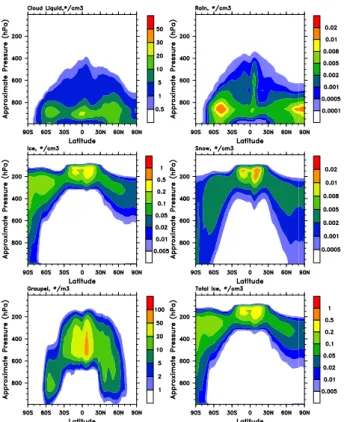
Figures 1 and 2 show annual average zonal mean latitude-pressure cross sections for grid-averaged hydrometeor mass and number concentrations, respectively. Simulated 20

cloud liquid water mass concentrations peak over the tropics and mid-latitude storm tracks at 800–900 hPa, which is similar to that of liquid droplet number concentrations, though the latter demonstrates the stronger influence of anthropogenic aerosols as cloud droplet number concentrations are higher in the Northern Hemisphere (NH) than in the Southern Hemisphere (SH). Rain water is more concentrated over the tropics, 25

(12)

ACPD

11, 3399–3459, 2011

M. Wang et al.

Title Page

Tables Figures

◭ ◮

Back Close

Full Screen / Esc

Discussion

P

a

per

|

Dis

cussion

P

a

per

|

Discussion

P

a

per

|

Discussio

n

P

a

per

|

dominated by warm collision-coalescence processes and drizzle from low clouds rather than melting from graupel and snow, which leads to low rain mass mixing ratios and high rain droplet number concentrations.

Simulated cloud ice mass concentrations peak in the upper troposphere over the tropics, while ice crystal number concentrations peak over both the tropics and high 5

latitudes because of colder temperatures over these regions. Snow water mass domi-nates the total ice water in the MMF model, as we discussed in Sect. 3.1, and graupel has a small contribution to the total ice water. The total ice water distribution shows a peak at 400–500 hPa over the tropics, and two other peaks over the mid-latitude storm track regions, which are in reasonable agreement with the total ice water distribution 10

from CloudSat (Waliser et al., 2009; Gettelman et al., 2010). The spatial distributions of the di_fferent ice hydrometeors are qualitatively similar to those from the NASA fvMMF (Fig. 12 in Waliser et al., 2009), except that the NASA fvMMF simulates a large contri-bution from graupel.

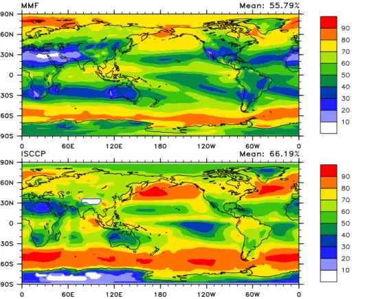
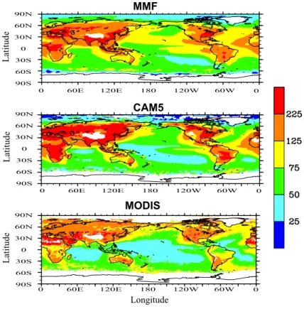
Figure 3 compares simulated annual mean total cloud cover with the ISCCP observa-15

tions. The total cloud cover in the MMF is diagnosed based on column-integrated total cloud water path (liquid+ice) at each CRM column. Columns are considered cloudy if the total cloud water path is larger than 1 g m−2 _{and clear otherwise. The}

instanta-neous total cloud cover is defined as a ratio of cloudy columns to the total number of columns in the CRM (32 in the current setup). The simulated spatial pattern of total 20

cloud cover is in reasonable agreement with observations, but in general, the model un-derestimates cloud fraction. The underestimation is especially true over regions where low clouds dominate, such as over the subtropical regions in which trade cumulus and stratocumulus are observed. This underestimation was also evident in several previ-ous MMF studies (Khairoutdinov et al., 2005, 2008). This is caused in part by the the 25

(13)

ACPD

11, 3399–3459, 2011

M. Wang et al.

Title Page

Tables Figures

◭ ◮

Back Close

Full Screen / Esc

Discussion

P

a

per

|

Dis

cussion

P

a

per

|

Discussion

P

a

per

|

Discussio

n

P

a

per

Figure 4 compares simulated annual mean shortwave and longwave cloud forcings with those from the CERES observations. Shortwave (longwave) cloud forcing is de-fined as the di_fference between the shortwave (longwave) clear-sky and all-sky radia-tive fluxes at the top of the atmosphere. Annual global mean shortwave cloud forcing in the MMF model is larger than the CERES observation (−0.5 vs.−47.1 W m−2). The 5

MMF model underestimates shortwave cloud forcing over regions with a large amount of low clouds, such as over the subtropical regions, consistent with the underestimation of cloud cover (Fig. 3), while it overestimates shortwave cloud forcing over the tropics. The longwave cloud forcing in the MMF model is smaller than the CERES observa-tion (26.0 vs. 29.9 W m−2). The radiative effect of snow particles is accounted for in 10

this study, and is included in the cloud forcing. A sensitivity test with the MMF model at a coarse GCM resolution (4◦

×5◦) shows that including the radiative effect of snow

increases the shortwave cloud forcing by about 8 W m−2 (in the absolute amount) and the longwave cloud forcing by 5 W m−2_{in January.}

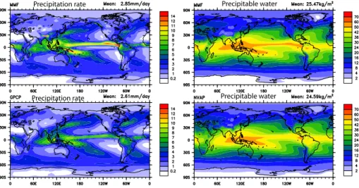
Figure 5 compares simulated annual-mean precipitation rate and precipitable wa-15

ter with observations. The model reproduces the overall features of the observation. However, the model simulates excessive precipitation over the West Indian Ocean, the Maritime continent, Australia, West Pacific, and East Pacific in the tropics, and West China. The model underestimates precipitation rate over ocean and over land in the subtropics and mid-latitudes. The simulated precipitable water has a similar pattern 20

as that in the observations. However, the model overestimates precipitable water over most of the oceans and the Maritime Continent, and underestimates precipitable water over land in the subtropics. The simulation of precipitation and precipitable water by this version of the MMF model is quantitatively similar to the previous version of MMF (Khairoutdinov et al., 2008). The two-moment cloud microphysics coupled with a modal 25

aerosol treatment in this version of the model does little to improve the simulations of precipitation and precipitable water.

(14)

ACPD

11, 3399–3459, 2011

M. Wang et al.

Title Page

Tables Figures

◭ ◮

Back Close

Full Screen / Esc

Discussion

P

a

per

|

Dis

cussion

P

a

per

|

Discussion

P

a

per

|

Discussio

n

P

a

per

|

4 of the MODIS by Quaas et al. (2006). For both the satellite and model data, only warm (>273 K) and low level clouds (pressure>640 hPa) are sampled. For consis-tency, the model output is only sampled at the satellite overpass time (13:30 LST). The MMF model reproduces the spatial patterns of the observed cloud-top droplet number concentrations, with larger droplet number concentrations over land than over 5

ocean and over the NH than over the SH, which clearly demonstrates the influence of anthropogenic aerosols. The patterns in gradients are replicated by both the MMF model as well as observations from the anthropogenic sources over land to its down-wind sides over marine environments, e.g., Pacific, Atlantic, and Indian Ocean. The MMF model also simulates enhanced droplet number concentrations over the South-10

ern Ocean (around 50◦_{S), consistent with MODIS observations. However, the MMF}

model overestimates droplet number concentrations over many oceanic regions, such as the Indian Ocean, the tropical Atlantic Ocean and the tropical Pacific Ocean. In con-trast, over the oceanic regions, CAM5 simulates fewer cloud droplets than the MMF, and agrees better with the MODIS observations. On the other hand, over the conti-15

nental regions, CAM5 simulates more cloud droplets than the MMF and overestimates cloud droplet number concentrations compared with the MODIS observations. The dif-ferences in simulated cloud-top droplet number concentrations between CAM5 and the MMF are consistent with the differences in simulated CCN concentrations discussed in Sect. 3.2.

20

3.2 Aerosol fields

Simulated aerosol fields in the present day simulation at a coarse GCM horizontal resolution (4◦×5◦) were documented and evaluated against observations in Wang et

al. (2010), and here we briefly compare the MMF results with CAM5.

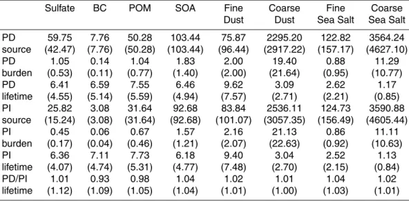
The annual, global mean aerosol sources, burdens, and lifetimes are summarized in 25

(15)

ACPD

11, 3399–3459, 2011

M. Wang et al.

Title Page

Tables Figures

◭ ◮

Back Close

Full Screen / Esc

Discussion

P

a

per

|

Dis

cussion

P

a

per

|

Discussion

P

a

per

|

Discussio

n

P

a

per

shown). The lower sulfate burden in CAM5 is partly from a larger wet removal rate, as evident from its shorter lifetime, and partly from smaller sulfate production (42.5 Tg S/yr in CAM5 vs. 59.8 Tg S/yr in the MMF). The latter is caused in part by the difference in the treatment of soluble fraction of SO₂. The soluble fraction of SO₂for wet removal is similar to that of H₂O₂in CAM5, which is quite e_fficient and leads to strong wet removal 5

of SO₂, while the soluble fraction of SO₂ in the MMF is based on the effective Henry law equilibrium and is much smaller than that of H₂O₂, resulting in less wet removal of SO₂. It is not surprising that sea salt and dust burden are similar in the MMF and CAM5 since dust and sea salt emissions in the MMF are tuned so their burdens match the CAM5 burdens.

10

Figure 7 shows aerosol size distributions in the marine boundary layer. The obser-vational data are from Heintzenberg et al. (2000) and were compiled and aggregated onto a 15◦×15◦ grid. The model output is sampled over the same regions as those

of observations. Aerosol size distributions simulated by both the MMF and CAM5 are in reasonable agreement with observations, and show bimodal distributions in most 15

regions. However, both the MMF and CAM5 underestimate the accumulation mode aerosol number concentrations, especially over the low and mid-latitude bands. This may suggest that the models underestimate fine-mode sea salt, polluted outflow from continents or the growth of Aitken mode particles. Wang et al. (2009) showed that the underestimation of fine-mode sea salt particles in their model was consistent with 20

their underestimation of accumulation mode aerosol number concentrations. Simu-lated aerosol number concentrations in the MMF are higher than that in CAM5 and agree better with observations. Higher aerosol number concentrations in the MMF are consistent with its higher global aerosol burdens (Table 2).

Figure 8 shows monthly BC concentrations at four sites in the polar regions. BC 25

(16)

ACPD

11, 3399–3459, 2011

M. Wang et al.

Title Page

Tables Figures

◭ ◮

Back Close

Full Screen / Esc

Discussion

P

a

per

|

Dis

cussion

P

a

per

|

Discussion

P

a

per

|

Discussio

n

P

a

per

|

the MMF demonstrate a similar improvement over CAM5 (not shown).

Figure 9 show the annual mean global distribution of CCN concentrations (at 0.1% supersaturation) averaged over the lowest 8 model levels (surface to about 800 hPa) in both the MMF and CAM5. The spatial patterns of CCN concentrations are similar in the MMF and CAM5, with high concentrations over strongly polluted regions, and low 5

concentrations over remote regions. However, the MMF produces lower CCN concen-trations in the strongly polluted regions and higher CCN concenconcen-trations in the remote regions, such as remote oceanic regions and polar latitudes, than CAM5. The higher CCN concentrations in the polar latitudes in the MMF can also be seen in the annual zonal distribution shown in Fig. 10, which is consistent with higher aerosol concentra-10

tions in the polar latitudes discussed above (Fig. 8). It is also evident in Fig. 10 that the MMF produces higher CCN concentrations at high altitudes than CAM5.

4 Aerosol indirect effects

4.1 Aerosol-cloud relationships in the PD

Following Quaas et al. (2009), the strength of aerosol-cloud interactions (ACI) is de-15

fined as the relative change in cloud properties with respect to the relative change in aerosol optical properties, and is calculated as:

ACI₌dlnC dlnA,

whereCis a cloud parameter (e.g., cloud droplet number concentration, cloud LWP, or cloud fraction), andAis a proxy for column-integrated aerosol number concentrations. 20

(17)

ACPD

11, 3399–3459, 2011

M. Wang et al.

Title Page

Tables Figures

◭ ◮

Back Close

Full Screen / Esc

Discussion

P

a

per

|

Dis

cussion

P

a

per

|

Discussion

P

a

per

|

Discussio

n

P

a

per

the particle size with smaller Angstrom coefficients for larger size particles. Here both AOD and AI are used as proxies for the column-integrated aerosol number concentra-tions to calculate ACI in the MMF model for cloud droplet number concentraconcentra-tions, LWP, and cloud fraction, following the same approach as that used in Quaas et al. (2009). ACI is obtained by a linear regression between lnC and lnA. Model output is sam-5

pled daily at 1:30 p.m. LT to match the MODIS Aqua equatorial crossing time. The model output is interpolated to a 2.5◦×2.5◦regular longitude-latitude grid as in Quaas

et al. (2009), to facilitate the direct comparison between the current study and Quaas et al. (2009). The regressions for the MMF and CAM5 simulations are performed sep-arately for fourteen different ocean and land regions and four seasons as in Quaas 10

et al. (2009). We compare the MMF results with those from the standard CAM5, and those from the observations and other model results in Quaas et al. (2009).

Figure 11 shows the mean sensitivities of cloud parameters to column aerosol prop-erties for all seasons in both the land and ocean areas from the satellite data, and from the MMF and CAM5 simulations, with the error bars showing the variability among 15

6 land or 8 ocean regions and 4 seasons. Cloud-top droplet number concentration increases with increasing AOD in both models and satellite observations (Fig. 11a). Simulated slopes between cloud-top droplet number concentration and AOD are simi-lar in the MMF and CAM5, with a slightly simi-larger slope in the MMF, and are significantly larger than that in satellite observations. Quaas et al. (2009) showed that most global 20

climate models overestimated the slope. Replacing AOD with AI in the MMF and CAM5 further increases the slope, which is consistent with McComiskey et al. (2009).

The slope between LWP and AOD is positive over land in the MMF model, consistent with those in satellite observations and CAM5, but the magnitude is larger in the MMF than in the satellite observations and in CAM5. In contrast, LWP and AOD over ocean 25

(18)

ACPD

11, 3399–3459, 2011

M. Wang et al.

Title Page

Tables Figures

◭ ◮

Back Close

Full Screen / Esc

Discussion

P

a

per

|

Dis

cussion

P

a

per

|

Discussion

P

a

per

|

Discussio

n

P

a

per

|

et al., 2005; Matsui et al., 2006). Using a global CRM with on-line aerosols, Suzuki et al. (2008) also obtained a negative correlation between LWP and AOD from a 8-day integration in July. The positive correlation between LWP and AOD is attributed to cloud lifetime effects or/and aerosol swelling effects in the high relative humidity regions surrounding clouds. The negative correlation between LWP and AOD can be 5

attributed to rain wash-out effects (Suzuki et al., 2004), semi-direct effects (Hansen et al., 1997), or dynamical feedbacks such as enhanced entrainment of drier air or enhanced evaporation of the more numerous smaller cloud droplets in polluted clouds (Ackerman et al., 2004; Jiang et al., 2006). Our results suggest that the negative effect dominates over ocean while the positive effect dominates over land in the MMF model. 10

Simulated cloud fraction and AOD are negatively correlated in the MMF and CAM5, opposite to the correlation found in the satellite retrievals, though using AI instead of AOD leads to a slightly positive correlation over land in both models. The positive correlation in satellite data can be attributed to the swelling of aerosol particles near clouds, cloud lifetime e_ffects, or the contamination in AOD retrievals by clouds. Quaas 15

et al. (2010) showed that the positive correlation between cloud fraction and AOD in their model can largely be attributed to the aerosol swelling e_ffects, and a negative correlation is found when dry AOD is used. The negative correlation between cloud fraction and AOD in CAM5 and the MMF may indicate the stronger scavenging effects of clouds on aerosols and/or less swelling e_ffects of clouds on aerosols in both models. 20

We noted that the MMF AOD is from the clear-sky CRM columns and therefore may be less susceptible to the swelling effects than CAM5 AOD.

4.2 Anthropogenic aerosol effects

4.2.1 Anthropogenic aerosol e_ffects in the MMF

As summarized in Table 2, simulated aerosol loadings have increased significantly 25

(19)

ACPD

11, 3399–3459, 2011

M. Wang et al.

Title Page

Tables Figures

◭ ◮

Back Close

Full Screen / Esc

Discussion

P

a

per

|

Dis

cussion

P

a

per

|

Discussion

P

a

per

|

Discussio

n

P

a

per

are similar in both PI and PD simulations. The lifetimes of sulfate, SOA, dust and sea salt increase slightly from PI to PD, which may be caused in part by cloud lifetime e_ffects (more aerosols lead to longer cloud lifetime, and therefore less efficient wet removal in PD than in PI), a positive feedback in aerosol indirect effects. On the other hand, the lifetimes of BC and POM decrease from PI to PD, which may be caused in part by 5

enhanced sulfate coating on BC and POM and therefore enhanced wet removal of BC and POM in the PD.

Figure 12 shows the global distribution of changes in annual-mean cloud-top droplet number concentrations and cloud-top droplet effective radius between the PD and the PI simulations (PD–PI). Cloud-top droplet number concentrations increase from the 10

PI to PD simulations over most regions, and increases in cloud-top droplet number concentrations are mainly located in the source regions of fossil fuel burning (e.g., more than 50 cm−3in Europe, East and South Asia) and biomass burning (e.g., more than 30 cm−3_{in Africa and South America), and downwind of the source regions (e.g.,}

between 10–30 cm−3 _{in the mid-latitude Pacific and the tropical Atlantic). Decreases} 15

in droplet number concentrations are simulated in some regions, such as Southeast United States, Central South America, and North Australia, which are caused by re-duced biomass burning emissions from PI to PD (not shown). Cloud-top droplet e_ff ec-tive radius decreases from the PI to PD simulations over most regions, by more than 1 µm over strongly polluted regions (e.g., East and South Asia) and more than 0.5 µm 20

over many oceanic regions (e.g., the North Pacific). The spatial pattern of changes in droplet effective radius is consistent with the spatial pattern of changes in cloud-top droplet number concentrations (i.e., large increases in droplet number concentrations lead to large decreases in droplet e_ffective radius).

Figure 13 shows the zonal distribution of changes in AOD, cloud liquid water 25

(20)

ACPD

11, 3399–3459, 2011

M. Wang et al.

Title Page

Tables Figures

◭ ◮

Back Close

Full Screen / Esc

Discussion

P

a

per

|

Dis

cussion

P

a

per

|

Discussion

P

a

per

|

Discussio

n

P

a

per

|

north of 30◦_{S, and peak in the NH mid-latitude with a value of about 0.04. Increases}

in cloud-top droplet number concentrations closely follow the changes in AOD, with a peak of about 40 cm−3in the NH mid-latitudes. Decreases in cloud-top droplet effective radius are larger over the NH mid-latitude, consistent with the large increases in cloud-top droplet number concentration, and also larger over the NH high latitudes, which can 5

be explained by the large relative changes in cloud-top droplet number concentrations. Increases in LWP are large over the tropics and the NH mid-latitudes, which is consis-tent with the increases in cloud droplet number concentrations over these regions. On the other hand, changes in LWP in the NH subtropics and the latitude bands around 60◦_{N are small though changes in cloud-top droplet number concentrations are large}

10

over these regions. Increases in the shortwave cloud forcing (in the absolute amount) are caused by both decreases in droplet effective radius and increases in LWP, while its changes follow more closely with changes in LWP than with changes in droplet ef-fective radius (e.g., smaller changes in the NH subtropics, and around 60◦_{N). Changes}

in net total fluxes at the top of the atmosphere are larger in the NH than in the SH. 15

The global mean changes from the PI to PD simulations are summarized in Table 3. Globally, anthropogenic aerosols lead to a 0.024 increase in clear-sky AOD, 24 cm−3

increase in cloud-top droplet number concentrations, a 0.53 µm decrease in cloud-top droplet effective radius, and a 2.10 g m−2 _{increase in LWP. A cooling of 0.77 W m}−2 _in

shortwave cloud forcing is simulated, which results from the decreases in cloud droplet 20

effective radius and increases in liquid water path. As expected, simulated longwave cloud forcing has little change between the PD and PI simulations since aerosol effects on ice clouds are not accounted for in this version of the MMF model. Simulated total aerosol effect on the shortwave fluxes at the top of the atmosphere is −1.31 W m−2.

Aerosol effect in the clear-sky (assuming entirely clear grid boxes) is −0.54 W m−2. 25

Simulated aerosol e_ffect on the net total fluxes (shortwave₊longwave) is₋1.05 W m−2_,

(21)

ACPD

11, 3399–3459, 2011

M. Wang et al.

Title Page

Tables Figures

◭ ◮

Back Close

Full Screen / Esc

Discussion

P

a

per

|

Dis

cussion

P

a

per

|

Discussion

P

a

per

|

Discussio

n

P

a

per

thermal emission from land.

4.2.2 Comparison with CAM5

In the standard version of CAM5, simulated PI to PD changes in shortwave cloud forcing, changes in longwave cloud forcing, aerosol direct effects in the clear sky (as-suming entirely clear grid boxes), and total aerosol effects are−1.79, 0.37,−0.45, and 5

−1.66 W m−2, respectively. A larger clear-sky direct effect in the MMF than in CAM5 (−0.54 W m−2 in the MMF vs.−0.45 W m−2 in CAM5) can be explained in part by the

larger increase in sulfate burden from PI to PD in the MMF (0.60 Tg S) than in CAM5 (0.36 Tg S). We also noted that aerosol water uptake in the MMF is calculated at each CRM grid cell with a CRM-scale relative humidity, while aerosol water uptake in CAM5 10

is calculated at each GCM grid cell with a GCM-grid scale clear-sky relative humidity. This may be another reason why the MMF simulates the larger clear-sky direct e_ffects, as previous studies (Haywood et al., 1997) showed that including subgrid variations in the relative humidity can lead to larger aerosol direct effects because of the nonlinear dependence of aerosol water uptake on relative humidity.

15

The simulated change in shortwave cloud forcing in the MMF (₋0.77 W m−2_{) is much}

smaller than that in CAM5 (−1.79 W m−2), despite the fact that changes in AOD and

cloud-top droplet e_ffective radius from anthropogenic aerosols in the MMF are slightly larger than those in CAM5 (Table 3 and Figs. 12, 13). For example, the global, annual mean change in cloud-top droplet effective radius is−0.53 µm in the MMF simulations, 20

compared with−0.45 µm in the CAM5 simulations (Table 3 and Fig. 12).

On the other hand, the smaller change in shortwave cloud forcing in the MMF is consistent with its smaller change in liquid water path (LWP) between the PI and PD simulations. Globally, an increase of 3.9% in LWP from PI to PD is simulated in the MMF, which is about one-fourth of the change of 15.6% in LWP in large-scale clouds 25

(22)

ACPD

11, 3399–3459, 2011

M. Wang et al.

Title Page

Tables Figures

◭ ◮

Back Close

Full Screen / Esc

Discussion

P

a

per

|

Dis

cussion

P

a

per

|

Discussion

P

a

per

|

Discussio

n

P

a

per

|

Continent, and Europe) and increases by more than 20% over some oceanic regions such as the North Pacific Ocean (Fig. 14). In contrast, the increase in LWP in the MMF is much weaker, less than 30% over most continental regions, and less than 10% over most oceanic regions. The scatter plots of the relative change in LWP and in shortwave cloud forcing shown in Fig. 15 further demonstrate that the larger change in LWP in 5

CAM5 leads to the larger change in shortwave clouds forcing. Zonal distributions of aerosol indirect effects in Fig. 13 also suggest that the large differences in simulated aerosol indirect e_ffects between the MMF and CAM5 occur over the regions where the difference in changes in LWP are larger such as the NH subtropics (compare Fig. 13b and e).

10

To further examine how clouds with di_fferent LWP may respond di_fferently to anthro-pogenic aerosols, Fig. 16 shows the probability density function (PDF) of in-cloud LWP over the globe in the PD simulations and the relative changes in the PDF of in-cloud LWP from the PI to PD simulations in both the MMF and CAM5. Model output (34 months data for the MMF and 4 years data for CAM5) are sampled daily at 1:30 p.m. 15

LT. For the MMF model, the PDF of LWP is calculated from in-cloud LWP at each CRM column (Fig. 16b and solid line in Fig. 16a) and at each GCM column (Fig. 16c and dotted line in Fig. 16a). For CAM5, the PDF of LWP is calculated from in-cloud LWP at each GCM column (Fig. 16d and dash-dot line in Fig. 16a). The in-cloud LWP in CAM5 is derived from grid-mean LWP, and liquid cloud cover that is calculated based 20

on the same maximum/random cloud overlap assumption used in the radiative transfer calculation in CAM5. The PDFs of LWP calculated from in-cloud LWP at each GCM column in both the MMF and CAM5 (Fig. 16c and d) are weighted by cloud cover. In-cloud LWP in CAM5 includes contribution from large-scale In-clouds only, while in-In-cloud LWP in the MMF includes contributions from both large-scale and convective clouds. 25

The PDFs of LWP in PD show that the frequency of occurrence of LWP decreases with increasing LWP and that clouds with LWP larger than 200 g m−2 _{occur more often in}

(23)

ACPD

11, 3399–3459, 2011

M. Wang et al.

Title Page

Tables Figures

◭ ◮

Back Close

Full Screen / Esc

Discussion

P

a

per

|

Dis

cussion

P

a

per

|

Discussion

P

a

per

|

Discussio

n

P

a

per

The relative changes in the PDF of LWP (green lines in Fig. 16b–d) show that cloud fraction of thin clouds decreases and that cloud fraction of thick clouds increases in both the MMF and CAM5 from the PI to PD simulations (relative changes in the frequency of occurrence of a given LWP bin is equivalent to relative changes in cloud fraction for that given LWP bin). It is also evident in Fig. 16b–d that cloud fraction increases in thick 5

clouds accelerate with increasing LWP bins. For example, in the MMF, cloud fraction decreases for clouds with in-cloud LWP less than 80 g m−2 and increases otherwise. For the smallest LWP bins, the decreases in cloud fraction can reach as high as 2%, while the increase in cloud fraction can be larger than 10% for clouds with LWP larger than 1000 g m−2. When the PDF of LWP is calculated from the in-cloud LWP at each 10

GCM column in the MMF (Fig. 16c), the di_fference between thin and thick clouds is even larger. The decreases in cloud fraction can reach as high as 4% for the smallest LWP bins, while the increase in cloud fraction can be larger than 10% for clouds with LWP larger than 350 g m−2_.

The di_fferent responses of thin and thick cloud LWP to anthropogenic aerosol pertur-15

bations can be explained in part by cloud lifetime effects. Thick clouds are more likely to precipitate and therefore their LWP are more susceptible to anthropogenic aerosol perturbations. The accelerating increase in cloud fraction for thick clouds with increas-ing LWP may partly result from the autoconversion scheme used in the models, which is based on Khairoutdinov and Kogan (2000). The autoconversion rate in Khairoutdi-20

nov and Kogan scheme has a strong dependence on liquid water content (q2_c.47), which leads to a strong dependence of the relative autoconversion rate (the autoconversion rate divided by liquid water content) on liquid water content (q1_c.47) and therefore larger relative increases in cloud fraction for clouds with larger LWP. On the other hand, thin clouds are less likely precipitating and their LWPs are therefore less susceptible to 25

(24)

ACPD

11, 3399–3459, 2011

M. Wang et al.

Title Page

Tables Figures

◭ ◮

Back Close

Full Screen / Esc

Discussion

P

a

per

|

Dis

cussion

P

a

per

|

Discussion

P

a

per

|

Discussio

n

P

a

per

|

Figure 16 shows that LWP changes are much larger in CAM5 than in the MMF. In CAM5, cloud fraction increases for clouds with in-cloud LWP less than 50 g m−2_{, and}

decreases otherwise. For the smallest LWP bins, the decrease in cloud cover is similar to that in the MMF, and can reach as high as 4%. On the other hand, for the larger LWP bins in CAM5, increase in cloud fraction is larger than 20% for clouds with LWP lager 5

than 200 g m−2, and is larger than 50% for clouds with LWP larger than 400 g m−2. The larger response in LWP in CAM5 can also be seen in the changes in the cumulative PDF of LWP (blue lines in Fig. 16b–d). In the MMF, total cloud fraction for clouds with LWP less than 300 g m−2decreases, and total cloud fraction for all LWP bins only slightly increases. In CAM5, total cloud fraction for clouds with LWP less than 70 g m−2 10

decreases, and total cloud fraction for all LWP bins increases by about 5%.

The cumulative LWP (red lines in Fig. 16b–d) shows that in-cloud LWP increases by less 4% in the MMF while it increases by about 10% in CAM5 (for a given LWP bin, the cumulative LWP is the in-cloud LWP averaged from the smallest LWP bin to the given LWP bin). These results are consistent with the grid-mean LWP changes shown 15

in Fig. 14. Changes in grid-mean LWP come from both changes in cloud fraction (the cumulative PDF) and in in-cloud LWP (the cumulative LWP). Figure 16 shows that the 3.9% increase in grid-mean LWP in the MMF is mainly from the changes in in-cloud LWP, while the 15.6% increase in large-scale LWP in CAM5 is from about 5% change in cloud fraction, and 10% change in in-cloud LWP.

20

Comparing changes in LWP (Fig. 14) with changes in CCN concentrations (Fig. 9), it is clear that changes in LWP in large-scale clouds in CAM5 closely follow changes in CCN concentrations. Large-scale LWP increases significantly over regions with large increases in CCN concentrations, such as East Asia and the Maritime Conti-nent. Compared with CAM5, increases in CCN concentrations in the MMF are weaker, 25

(25)

ACPD

11, 3399–3459, 2011

M. Wang et al.

Title Page

Tables Figures

◭ ◮

Back Close

Full Screen / Esc

Discussion

P

a

per

|

Dis

cussion

P

a

per

|

Discussion

P

a

per

|

Discussio

n

P

a

per

concentrations in CAM5 than in the MMF are consistent with the changes in aerosol lifetimes between the PD and PI simulations (Table 2). The lifetime of sulfate aerosol is almost the same in the PD and PI simulations in the MMF, but increases by 12% from the PI to PD simulations in CAM5. The lifetime of BC decreases by 7% from the PI to PD simulations in the MMF, while it increases by 9% in CAM5. The large increase 5

in sulfate and BC lifetimes in CAM5 from the PI to PD simulations can be explained in part by the positive feedback in aerosol indirect effects due to cloud lifetime effects (more aerosols lead to longer cloud lifetime and therefore less wet scavenging, which in turn increases CCN concentrations). Our results indicate that this positive feedback induced by cloud lifetime effects is stronger in CAM5 than in the MMF, and can partly 10

explain the stronger changes in shortwave cloud forcing in CAM5 due to anthropogenic aerosol perturbations.

Comparing changes in LWP (Fig. 14) with changes in CCN concentrations (Fig. 9), it is also clear that the MMF produces more regions with negative response in LWP to anthropogenic aerosols than CAM5. For example, though CCN concentrations in-15

crease significantly from the PI to PD simulations over South China, LWP changes little or even decreases in the MMF, while it increases significantly in CAM5. Figure 16 also shows that negative changes in cloud fraction extend to thicker clouds in the MMF than in CAM5. This indicates that factors other than the differences in the relative changes in CCN concentrations are also important in causing the smaller increase in LWP in 20

the MMF model.

Figure 17b and c compare the relative changes in CCN concentrations with the rela-tive changes in LWP in both the MMF and CAM5, respecrela-tively. It is clear that the much smaller increase in LWP in the MMF is caused primarily by the much smaller response in LWP to a given change in CCN. The slope between the relative change in LWP and 25

(26)

ACPD

11, 3399–3459, 2011

M. Wang et al.

Title Page

Tables Figures

◭ ◮

Back Close

Full Screen / Esc

Discussion

P

a

per

|

Dis

cussion

P

a

per

|

Discussion

P

a

per

|

Discussio

n

P

a

per

|

cloud droplets, which results in less precipitation, larger LWPs and longer cloud life-times (Albrecht, 1989). However, ship track studies show that anthropogenic aerosols can lead to less liquid water (Platnick et al., 2000; Coakley and Walsh, 2002), and satellite studies show both decreases and increases in LWP with increasing aerosols (Kaufman et al., 2005; Matsui et al., 2006). CRM studies have suggested that LWP 5

can either increase or decrease with increasing aerosols, depending on the meteoro-logical conditions (Ackerman et al., 2004; Jiang et al., 2006; Guo et al., 2007; Xue et al., 2008; Small et al., 2009). The decreasing LWP with increasing aerosols can be attributed to enhanced entrainment of dry air or enhanced evaporation of the more nu-merous smaller cloud droplets in polluted clouds. Stevens and Feingold (2009) further 10

argued that the aerosol-cloud interactions work in a bu_ffered system, and cloud lifetime e_ffects as hypothesized in the system in isolation may be canceled or compensated for by opposing changes when the system is viewed as a whole. Most conventional global climate models implemented cloud lifetime e_ffects through their large-scale cloud pa-rameterization and are not able to account for the sophisticated balance between di_ff er-15

ent factors, and hence may overestimate cloud lifetime effects. Compared with CAM5, the smaller increase in LWP in the MMF model is more consistent with the observations and with CRM studies.

4.2.3 Comparison with other studies

The smaller increase in LWP in the MMF model is consistent with Lohmann (2008), who 20

showed a slightly smaller response in LWP in a version of the ECHAM including aerosol e_ffects on convective clouds using cumulus parameterization (8.2%) compared to a version of the ECHAM without aerosol effects on convective clouds (9.7%) though con-ventional cloud parameterizations are used for both stratiform and convective clouds. In Lohmann (2008), the total aerosol e_ffect decreases slightly from₋1.9 W m−2_without

25

aerosol effects on convective clouds to−1.7 W m−2 with aerosol effects on convective

(27)

ACPD

11, 3399–3459, 2011

M. Wang et al.

Title Page

Tables Figures

◭ ◮

Back Close

Full Screen / Esc

Discussion

P

a

per

|

Dis

cussion

P

a

per

|

Discussion

P

a

per

|

Discussio

n

P

a

per

when aerosol effects on convective clouds are included. In contrast, the CSIRO model in Menon and Rotstayn (2006) simulates a larger increase in LWP when aerosol e_ffects on convective clouds are included. Menon and Rotstayn (2006) attributed the different responses in the CSIRO and GISS models to the different treatment of detrained con-densate in their cumulus parameterizations, which includes di_fferent treatments on how 5

to partition convective condensate into precipitation and detrained condensate, and on how to treat detrained cloud condensate (instantly evaporate in CSIRO, and is added directly as anvil clouds in GISS). It is not clear in Menon and Rotstayn (2006) why these differences lead to different responses in liquid water path to anthropogenic aerosols in the two models.

10

The estimated shortwave cloudy-sky forcing, calculated from subtracting aerosol ef-fects in the clear sky weighted by the clear-sky fraction from the total shortwave forcing, is−1.07 W m−2, which is at the low end of the estimates of global aerosol-climate

mod-els included in a recent AeroCom indirect e_ffect model intercomparison study (Quaas et al., 2009). The estimated shortwave cloudy-sky forcing in Quaas et al. (2009) range 15

from −0.27 to −1.87 W m−2 with a mean value of −1.15 W m−2 though none of the

participated AeroCom models included aerosol indirect e_ffects on convective clouds. The AeroCom models that produced small shortwave cloudy-sky forcing typically set a larger lower limit for simulated droplet number concentrations ranging from 20 to 40 cm−3_{. It has been shown in several previous studies (Ghan et al., 2001; Hoose et}

20

al., 2009; Wang and Penner, 2009) that the larger lower limits usually lead to smaller aerosol indirect effects. The CRM in the MMF model does not include any lower limit on simulated cloud droplet number concentrations, the same as CAM5 and several other models in Quaas et al. (2009) that generally produced larger shortwave cloudy-sky forcing.

25

The AeroCom models that produced low shortwave cloud-sky forcing also typically have a weak dependence of autoconversion rate on cloud droplet number concen-trations. For example, the smallest forcing in the AeroCOM models (−0.27 W m−2) is