Nonlin. Processes Geophys., 15, 575–590, 2008 www.nonlin-processes-geophys.net/15/575/2008/ © Author(s) 2008. This work is distributed under the Creative Commons Attribution 3.0 License.
Nonlinear Processes
in Geophysics
Quantification of tillage, plant cover, and cumulative rainfall effects
on soil surface microrelief by statistical, geostatistical and fractal
indices
J. Paz-Ferreiro1, I. Bertol2, and E. Vidal V´azquez1
1Faculty of Sciences, University of Corunna-UDC, Spain
2Soil and Natural Resources Department, University of Santa Catarina State-UDESC, Brazil
Received: 4 September 2007 – Revised: 17 June 2008 – Accepted: 18 June 2008 – Published: 23 July 2008
Abstract. Changes in soil surface microrelief with cumula-tive rainfall under different tillage systems and crop cover conditions were investigated in southern Brazil. Surface cover was none (fallow) or the crop succession maize fol-lowed by oats. Tillage treatments were: 1) conventional tillage on bare soil (BS), 2) conventional tillage (CT), 3) minimum tillage (MT) and 4) no tillage (N T) under maize and oats. Measurements were taken with a manual relief meter on small rectangular grids of 0.234 and 0.156 m2, throughout growing season of maize and oats, respectively. Each data set consisted of 200 point height readings, the size of the smallest cells being 3×5 cm during maize and 2×5 cm during oats growth periods. Random Roughness (RR), Lim-iting Difference (LD), Limiting Slope (LS) and two frac-tal parameters, fracfrac-tal dimension (D) and crossover length (l)were estimated from the measured microtopographic data sets. Indices describing the vertical component of soil rough-ness such asRR,LDandl generally decreased with cumu-lative rain in theBStreatment, left fallow, and in theCT and MTtreatments under maize and oats canopy. However, these indices were not substantially affected by cumulative rain in theN T treatment, whose surface was protected with previ-ous crop residues. Roughness decay from initial values was larger in theBStreatment than in CT andMT treatments. Moreover, roughness decay generally tended to be faster un-der maize than unun-der oats. The RR andLD indices de-creased quadratically, while thel index decreased exponen-tially in the tilled,BS,CT andMT treatments. Crossover length was sensitive to differences in soil roughness
condi-Correspondence to:E. Vidal V´azquez ([email protected])
tions allowing a description of microrelief decay due to rain-fall in the tilled treatments, although better correlations be-tween cumulative rainfall and the most commonly used in-dicesRRandLDwere obtained. At the studied scale, pa-rameterslandDhave been found to be useful in interpreting the configuration properties of the soil surface microrelief.
1 Introduction
The Earth’s topography encompasses a considerable range of scales. The horizontal scale of lithosphere relief varies from sizes smaller than millimeters to sizes as large as the planet with a perimeter in the order of 40 000 km (Huang, 1998; Lovejoy and Schertzer, 2007). The vertical scale of litho-sphere relief reaches some 18 km considering fluctuations between oceanic bed and continental mountains. Therefore, topography variability on our planet is higher than factors of over 1010 and 107 in the horizontal and vertical scales, re-spectively. At the planetary scale, topography remains rela-tively unchanged except in active volcanic and tectonic areas (Lovejoy and Schertzer, 2007).
Both landscape topography and soil surface microrelief are the result of many competing influences. However, un-like topography at the landscape scale, the microrelief can change rapidly in agricultural fields in response to tillage op-erations, erosion, deposition and other less dominant factors. Moreover, the roughness of the soil surface results from dif-ferent elements such as individual grains, aggregates, clods, tillage marks and landscape features that each contribute at various scale lengths. Conversely, soil roughness can be split into several components. First, surface variations due to the spatial distribution of individual grains, aggregates and clods, define random roughness. Second, systematic differ-ences in elevation caused by tillage implements such as fur-rows are referred to as oriented roughness; if concentrated erosion occurs, rills and gullies also contribute to oriented roughness. Third, at the field and landscape scales higher or-der roughness created by the general topographic slope with its concavities and convexities may be recognized; this type of roughness is the most interesting to sciences concerned with topographic or macrorelief scales (R¨omkens and Wang, 1986).
Soil surface roughness affects many transfer processes on and across the soil-atmosphere boundary, for example, infil-tration, runoff, soil detachment by water and wind, gas ex-change and evaporation. The temporal water storage in mi-crorelief depressions controls overland flow generation and runoff pathways (Hairsine et al., 1992; Hansen et al., 1999; Favis-Mortlock et al., 2000). The quantification of roughness related parameters such as depression storage is considered of great relevance and practical importance, because it can be used to enhance both water conservation and soil conser-vation.
Soil surface roughness can also act as an erosivity factor at smaller scales within a microplot, affecting the soil response to raindrop impact and other erosive forces, and as an erodi-bility factor at larger scales of the sizes of a plot, a field or a hillslope, affecting the origin and spatial organization of the drainage pattern (Merril et al., 2001). This demonstrates the interaction between the length scale of a physical process on the soil surface and the scale of roughness components.
Because the random roughness condition is initiated by the variable disposition of aggregates and clods on the soil surface roughness, it is associated to disordered microre-lief (Huang, 1998; Vidal V´azquez et al., 2005). Therefore, the term “random” only describes non-orderly distribution of structural unities on the soil surfaces and should not be misleading, since random roughness is spatially correlated at short distances (Linden and van Doren, 1986; Huang and Bradford, 1992; Helming et al., 1998; Eltz and Norton, 1997; Miranda, 2000; Zribi et al., 2000; Vidal V´azquez et al., 2005, 2006, 2007). This correlation seems to be a usual property of soil surface random roughness irrespective of soil type and tillage condition. The range of spatial dependence is of the same order of magnitude as the largest structural unities, aggregates and clods, on the soil surface. Above distances
larger than the main structural unities, correlation tends to disappear.
Oriented roughness can be easily quantified by determin-istic models, because it depends on slope and/or on a spe-cific tillage tool (Huang, 1998). In contrast, random rough-ness analysis has been more challenging, as it should include a characterization of the spatial structure of microrelief el-ements with various sizes. Soil surface roughness, however, has been most frequently described by the random roughness or the root mean square roughness index (Allmaras et al., 1966). This index is equivalent to the standard error of point elevations relative to a reference plane and represents a sta-tistical measure of vertical topographic fluctuation, implic-itly assuming that there is no spatial dependence in surface roughness. But its main shortcoming is that two soil surfaces with identical RR values may have different topographies (R¨omkens and Wang, 1986; Merril et al., 2001).
Furthermore, soil surface roughness, measured asRR, in-creases as the area extent of point elevation measurements is increased. Consequently, roughness should be expressed as a scale-dependent function, not merely as a statistical index (Huang, 1998). Different approaches have been proposed to account for the spatial scale. Based on the first order semi-variogram, i.e., elevation difference measure, Linden and van Doren (1986) defined two indices: limiting difference (LD) and limiting slope (LS), describing the vertical component and the separation length scale of soil surface roughness, re-spectively. Correlation and spectral density analysis have been used to quantify roughness and to examine roughness changes as a function of rain and tillage operations (Currence and Lovely, 1970; Dexter, 1977).
Fractal models have been used to describe not only the Earth’s topography (e.g. Mandelbrot, 1983; Lovejoy and Shertzer, 2007) but also soil microrelief (Armstrong, 1986; Huang and Bradford, 1992; Eltz and Norton, 1997; Huang, 1998; Miranda, 2000; Vidal V´azquez et al., 2005, 2006, 2007). The term “fractal” is often taken to be synonymous with “scale-invariance”, the well known property that many geologic and soil characteristics look the same at all scales. This is referred to as self-similarity. In a self-similar frac-tal the factor that characterizes the invariance is indepen-dent of the direction. However, a fractal is iindepen-dentified as self-affine when different scaling ratios are found for each inde-pendent direction. Early studies of Mandelbrot (1985) and Voss (1985) showed that the height of topography along a lin-ear track can only be self-affine and not self-similar. By ex-tension, topographic surfaces are also examples of self-affine fractals (Vidal V´azquez et al., 2005; Lovejoy and Shertzer, 2007).
J. Paz-Ferreiro et al.: Microrelief fractal parameters 577 models (Vidal V´azquez et al., 2005). It should be
empha-sized that non-variational techniques such as tortuosity eval-uation (Bertuzzi et al., 1990) and Richardson number (Gal-lart and Pardini, 1996; Pardini and Gal(Gal-lart, 1998; Pardini, 2003) are only appropriate for self-similar surfaces and there-fore they should not be applied for estimating fractal param-eters from point elevation data sets, which are self-affine. In contrast, variational models allow a description of soil sur-face microrelief from self-affine data sets. Because varia-tional and non-variavaria-tional models are not equivalent, results from both of these types of methods frequently do not agree (Miranda, 2000; Vidal V´azquez et al., 2005) and cannot be directly compared.
Two parameters are required to describe the scale de-pendent roughness function by a variational fractal model, namely fractal dimension,D, and crossover length,l. Frac-tal parameters, D andl, account for the multiscale effects and for the fluctuations of local vertical statistics, respec-tively (Huang and Bradford, 1992; Eltz and Norton, 1997; Huang, 1998; Miranda, 2000; Vidal V´azquez et al., 2005, 2007).
Soil surface roughness controls microrelief depression pat-tern and is clearly relevant to estimate depression storage ca-pacity (Huang and Bradford, 1990; Kamphorst et al., 2000; Darboux et al., 2005). Therefore, the scale dependence of soil microrelief has implications in modeling this parameter. However, most runoff and erosion processes are not affected by the short-distance correlation so they could be quantified by a single parameter, without taking into account these scale dependent function. In other words, fractal-based roughness parameters are not necessarily more important than other in-dicators, based on statistics or on geostatistics.
This paper aims to clarify the relevance of the fractal ap-proach for soil surface roughness evaluation. It extends pre-vious studies on data sets acquired with low technology de-vices, characterizing large scale surface features. The main focus is on soil management effects over initial roughness created during tillage operations and on roughness destruc-tion and decay by cumulative rainfall under a crop succes-sion.
2 Material and methods
2.1 Site, soil and tillage operations
This study was conducted at the agricultural research station of the University of the State of Santa Catarina (UDESC) in Lages, Santa Catarina State, Brazil, latitude 27◦49′S, lon-gitude 50◦20′W and mean altitude 937 m a.s.l. The climate was classified as Cfb type according to K¨oppen, with an av-erage yearly rainfall and erosivity of about 1600 mm and 6000 MJ mm ha−1h−1, respectively (Bertol et al., 2002a). The experimental area has been used for water erosion stud-ies under natural rainfall since November 1988. The data sets
for our study were acquired between May 2003 and October 2004.
The studied soil with a moderate A horizon and a silty-clay sedimentary bedrock, was classified as an Inceptisol (Soil Survey Staff, 1993). The topsoil (0–20 cm depth) is clay tex-tured, with 142 g kg−1 sand, 437 g kg−1silt and 421 g kg−1 clay contents. Bulk density in this layer was 1.28 kg dm−3. Soil erodibility was 0.0115 t ha h ha−1MJ−1mm−1(Bertol et al., 2002b) and the mean slope of the experimental plots was 0.10 m/m.
Field experiments were conducted during the growth period of two successive crops, maize and oats, using 3.5 m×22.1 m erosion plots. Tillage treatments were as fol-lows: 1) ploughing and two times harrowing on bare soil, as a control treatment (BS), 2) conventional tillage which consisted also of ploughing followed by two successive har-rowing (CT), 3) minimum tillage which consisted of chisel ploughing and harrowing (MT) and 4) no-tillage over pre-vious crop residues (N T). Tillage systems were in a ran-domized design, without replications. TreatmentsCT,MT andN T were cropped first to maize (Zea mays) and after to oats (Avena strigosa), both crops being a part of a multi-ple rotation system. Cumulative rain amounted to 229 mm and 350 mm in the growth periods of maize and oats, respec-tively. A detailed description of tillage operations and exper-imental setup was presented elsewhere (Bertol et al., 2002, 2006).
Operations with different tillage implements produced soil surfaces visibly different between treatments. In the conven-tionally tilled treatments (BSandCT) as well as in the min-imum tillage treatment (MT) a range of aggregates and clod sizes was observed. These structural elements were more or less evenly distributed in theBSandCT treatments. How-ever, in MT treatment rougher areas of disturbed soil due to chisel ploughing were distinct from undisturbed smoother areas between the chisel rows. Furthermore,CT andMT treatments were partly covered by previous crop residues that contributed to microrelief, because they were not to-tally incorporated into the soil by ploughing. Therefore, par-tial residue soil cover was larger inMT than inCT treat-ment. UnderN T soil surface microrelief consisted of undu-lated land without tillage marks, fully protected by free crop residues, covering the entire soil surface.
2.2 Field data sets and trend removal
Soil surface microrelief was measured five times in the maize growth season and four times in the oats growth season. The first measurement was made just at sowing time; then succes-sive readings were taken at about 15 days apart throughout each crop growth period.
measurements in the oats season were performed with nee-dles spaced 2 cm apart, along 78 cm transects. In both cases 5 profiles were taken per plot, 5 cm apart from each other. This gave 200 readings at any location. Therefore, the sampling scheme was a 3 cm×5 cm rectangular grid when the soil was cropped to maize and it was a 2 cm×5 cm grid in the oats sea-son. The area of the roughness experimental plot was 0.234 and 0.156 m2in the maize and oats crops, respectively. For each transect, the pin position was registered photographi-cally and later digitized to record readings of 40 calibrated needles, as described by Wagner and Yiming Yu (1991).
Manual pinmeters are destructive devices. Thus, different microplots were used for surface roughness measurements at increasing amounts of cumulative rainfall in successive dates. Within each tillage treatment, experimental plots were located as close as possible to minimize the effect of spatial variability between them.
Microrelief data sets were corrected for slope and tillage marks. Correction for slope was obtained using the plane of best fit to the 200 point elevation readings of each plot. Ad-ditionally, non-directional random roughness surfaces were obtained by removing row and column effects, as proposed by Currence and Lovely (1970). Therefore, all the indices in this study were estimated for data sets representing the ran-dom roughness condition.
The configuration of soil topography was simple described by a set of points of knownx-,y- andz-coordinates. The ele-vation values given as a function of the horizontal coordinate system provide a numerical representation of the surface and constitute a digital elevation model (DEM). From each ex-perimental data set of soil surface microtopography a DEM was obtained after trend removal, representing the random roughness condition.
2.3 Statistical and geostatistical indices
Besides quantifying of fractal parameters, in this study three traditional roughness indicators were assessed: a statistical index, random roughness (RR), and two geostatistical in-dices estimated from the first order semivariogram of point elevation differences, referred to as “limiting difference” (LD) and “limiting slope” (LS).
In accordance with Currence and Lovely (1970) and Kam-phorst et al. (2000),RRwas estimated simply as the stan-dard deviation of height readings after correction for slope and tillage marks. Therefore, in this studyRRwas assessed without a log-transformation of the residual point elevation data and without removing extreme values, as initially pro-posed by Allmaras (1966). Random Roughness was calcu-lated as:
RR= v u u u t
n P
i=1
(Zi−Z)2
n (1)
whereZiandZare point elevation and mean point elevation, respectively, andnis the number of experimental points.
LDandLSquantification is based on the first-order vari-ogram of mean absolute differences in elevation (1Zh) sep-arated by a distance vector, h. Following Linden and van Doren (1986), the first step in estimatingLDandLSconsists in the computation of the mean absolute elevation difference, as:
1Zh = n X
i=1
|Zi −Zi+h|
n (2)
whereZi andZi+hare elevations at positions located a hor-izontal distancehapart andnis the number of data points. Therefore, for a two-dimensional data set,Zi+hcorresponds to point heights located in a disk of radii h around pointi.
Then, parameters, a andb, of the linear relationship be-tween 1/1Zhand 1/1hare estimated:
1 1Zh
= a + b 1Xh
(3) ParametersLDandLSare quantified, respectively, as:
LD = 1
a (4a)
LS = 1
b (4b)
The limiting difference,LD, is mathematically interpreted as the value of1Zwhenhapproaches large spatial intervals. The limiting slope,LS, is the slope or1Z/1h, whenh ap-proaches zero. This analysis is essentially independent of the minimum spacing interval because of the linear nature of Eq. (3).
In estimating roughness indices based on geostatistical concepts (LDandLS), surface microrelief was assumed to be statistically homogeneous, which implies that statistical properties do not depend on the position, but only depend on the spatial separation,h.
2.4 Fractal dimension and crossover length
A fractal analysis was performed on the soil microrelief data sets using a variational method, thus assuming a self-affine model for microrelief description. This method is based on a fractional Brownian motion (fBm) model to calculate the Hurst exponent,H, from which the fractal parametersDand lare obtained.
J. Paz-Ferreiro et al.: Microrelief fractal parameters 579 (Malinverno, 1990; Miranda, 2000). The semivariance can
be estimated from sampling data as:
γ×(h)= 1 2n
n X
i=1
[Z(xi+h)−Z(xi)]2 (5)
whereγ×(h) is known as the experimental semivariogram, nis the number of pairs of sample points of observations of the values of the studied attribute,Z, between any two places x andx+h, separated by a distanceh,Z(x) is the elevation at locationx.
Data sets were checked for the intrinsic hypothesis of the regional variable theory. After trend removal the two condi-tions defining the requirements for the intrinsic hypothesis, i.e., stationarity of differences and variance of differences were verified.
The use of the γ (h) function as the roughness measure gives a direct relationship between an elevation difference term and the separation length scale,h. This is an important step in fractal analysis as the estimated values of fractal pa-rameters,Dandlfrom soil topography surfaces or transects, may show some bias depending not only on the assumptions made in formulating the fractal model but also on the algo-rithm which is used (Miranda, 2000; Vidal V´azquez et al., 2005, 2006).
Burrough (1983 a,b) first used theγ(h) structural func-tion in soil science. The semivariance funcfunc-tion for estimat-ing fractal dimension of soil height tracks was introduced by Armstrong (1986) and later on applied to various surface types (Carr and Benzer, 1991; Davis and Hall, 1999), includ-ing agricultural soils (Huang and Bradford, 1992; Miranda, 2000; Vidal V´azquez et al., 2005, 2006, 2007).
The fractal model used for soil surface roughness quantifi-cation was the fractal Brownian motion model (fBm). The elevation difference of a fBm is given by:
(1Zh) ∝ hH,1> H >0 (6)
where the exponent of the incremental function, H, is the Hurst exponent. The power model, which describes a self-similar fractal, corresponds to a phenomenon with an unlim-ited capacity for spatial dispersion and with an a priori unde-fined variance.
In a fractal Brownian motion model (Eq. 6), the Hurst ex-ponent is allowed to vary from 0 to 1 (Huang and Bradford, 1992). A fBm is an expansion of the random walk or Brown-ian model (Bm) characterized by Hurst exponentH=0.5, first proposed by Mandelbrot and van Ness (1968). Conversely, the random walk or Bm model can be considered an especial case of the fBm.
For a fractal transect the semivariance function, accord-ing to Mandelbrot (1983, p. 353), is a function of the spatial separation:
γ (h)∝h2H (7)
The fractal dimension,D, of a fractal surface or profile repre-sented by its semivariogram can be estimated from the slope of the straight line portion of the semivariance, γ(h), ver-sus the lag distance,h, when plotted on a double logarithmic scale.
For a two dimensional data set of point heights, the fractal dimension,DSMV, is computed from the Hurst exponent,H,
obtained by Eq. (7), and the Euclidean dimension (d=3) as:
DSMV=3−H (8)
In addition to the commonly used fractal dimension,D, rameter, the fractal roughness model requires a second pa-rameter to define the relative position of the straight line of the variogram plotted on a log-log scale. Huang and Brad-ford (1990) defined this parameter as the crossover length,l, and it should be used together withDfor characterizing soil surface roughness at small distances. The semivariance func-tion of the fMb fractal model may be described as a funcfunc-tion of both, crossover length,l, and the exponent,H, as:
γ (h)=l2−2Hh2H (9)
In Eq. (9) γ (h)=h2 when h=l, which explains the origin of the term crossover length, first proposed by Huang and Bradford (1992) for soil microrelief quantification.
The crossover length,l, may be estimated from the slope of the straight line portion of a variogram by:
lSMV=exp[(a/2−2H )] (10)
wherea, is the intercept of the straight line of the semivari-ance log-log plot at the y-axis.
It follows that characterizing soil surface roughness by a fractal fBm model requires two parameters, fractal dimen-sion,D, and crossover length,l, as shown by theoretical con-siderations (Huang and Bradford, 1992) and by experimental results (Huang and Bradford, 1992; Eltz and Norton, 1997; Miranda 2000; Vidal et al., 2005).
3 Results and discussion
3.1 Statistical and geostatistical roughness indices
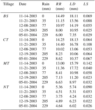
Table 1. Sampling date, cumulative rainfall, random roughness (RR), limiting difference (LD) and limiting slope (LS) during the maize season for different tillage treatments. (BS=bare soil, CT=conventional tillage,MT=minimum tillage,N T=no-tillage).
Tillage Date Rain RR LD LS
(mm) (mm) (mm)
BS 11-14-2003 0 14.49 18.11 0.069 11-21-2003 35 11.15 13.56 0.088 12-08-2003 77 10.97 14.19 0.055 12-19-2003 205 8.00 10.95 0.025 05-01-2004 229 6.00 7.35 0.029 CT 11-14-2003 0 14.25 18.13 0.064 11-21-2003 35 14.40 16.78 0.108 12-08-2003 77 10.02 13.06 0.053 12-19-2003 205 8.23 10.06 0.064 05-01-2004 229 8.62 10.37 0.067 MT 11-14-2003 0 13.00 15.79 0.142 11-21-2003 35 11.36 17.72 0.040 12-08-2003 77 8.41 10.98 0.058 12-19-2003 205 7.13 11.20 0.023 05-01-2004 229 6.63 8.97 0.032 N T 11-14-2003 0 5.36 5.74 0.090 11-21-2003 35 4.51 5.31 0.053 12-08-2003 77 3.75 4.24 0.032 12-19-2003 205 4.89 6.23 0.022 05-01-2004 229 4.64 6.02 0.026
Table 2. Sampling date, cumulative rainfall, random roughness (RR), limiting difference (LD) and limiting slope (LS) during the oats season for different tillage treatments. (BS=bare soil, CT=conventional tillage,MT=minimum tillage,N T=no-tillage).
Tillage Date Rain RR LD LS
(mm) (mm) (mm)
BS 08-18-2004 0 14.97 17.04 0.206 08-31-2004 50 11.81 11.56 0.090 09-17-2004 153 9.22 9.82 0.213 10-05-2004 350 5.77 8.79 0.013
CT 08-18-2004 0 8.02 9.66 0.137
08-31-2004 50 8.90 10.66 0.130 09-17-2004 153 8.41 9.73 0.144 10-05-2004 350 4.56 5.34 0.058
MT 08-18-2004 0 7.40 8.70 0.126
08-31-2004 50 6.36 7.75 0.112 09-17-2004 153 7.63 8.72 0.119 10-05-2004 350 5.32 6.34 0.070 N T 08-18-2004 0 12.12 14.25 0.135 08-31-2004 50 11.90 14.06 0.264 09-17-2004 153 11.22 13.14 0.144 10-05-2004 350 11.65 13.54 0.055
y = 0.906x - 0.49 R2 = 0.943
y = 0.748x + 0.38 R2 = 0.944
2 4 6 8 10 12 14 16 18 20
2 4 6 8 10 12 14 16 18 20
LD (mm)
RR
(m
m
)
maize oats
Fig. 1. Random roughness (RR) versus limiting difference (LD) indices as recorded during maize and oats seasons.
J. Paz-Ferreiro et al.: Microrelief fractal parameters 581 The relationship betweenRRandLDis shown in Fig. 1.
In our study the correlation coefficients between these in-dices were 0.944 and 0.943 for the 20 data sets acquired during the maize season and the 16 data sets acquired in the oats season, respectively. Both relationships were lin-ear and significant (P <0.01). Linden and van Doren (1986) and Bertuzzi et al. (1990) also found a linear relationship be-tween these two indices.
The limiting difference,LD=1/a, in Eq. (4a) is the asymp-tote value of the first-order semivariance, i.e. the sill of the first-order semivariogram. Indeed, RR corresponds to the square root of the sill of the second order semivariogram. Consequently strong correlation coefficients between RR andLD are expected. However, distinct regression equa-tions in the maize and oats seasons in our study together with previous results (Linden and van Doren, 1986; Bertuzzi et al., 1990) suggest that there is not a general relationship be-tween these two indices, in spite of its strong dependence for a given specific experimental condition. AlthoughRR andLD are indicators of the height distribution of surface microrelief, they do not account for the spatial component, i.e. mutual location of higher and lower points. Spatial struc-ture of the microtopography is critical for a thorough charac-terization of the configuration properties of the soil surface and for depressional storage evaluation.
Linden and van Doren (1986) stated thatLSis soil surface slope at small intervals, because1Z/1h would approachLS when1happroaches zero. Therefore,LSshould give infor-mation on the side slopes of structural units, such as large aggregates or clods, at small intervals. Moreover, on an ide-alized soil surface, maximum roughness depends on the side slope of the structural elements protruding the soil surface. The magnitude ofLS was small when compared with those ofRRorLD, as this index ranged from 0.013 to 0.264 in the oats season and from 0.022 to 0.142 in the maize season. In our study cases no significant correlation was found between LDorRRandLS.
Because of the linear nature of Eq. (3),LD andLS are essentially independent of the minimum sampling interval, which represent an advantage for analyzing data sets with various sampling grids. However, maximum soil surface roughness as assessed by theLD or the RRindices is in-dependent of the size of the structural elements at the soil surface, which means that two different surface configura-tions may result in the sameLDorRRvalues (Merril et al., 2001). This continues to be a major problem in characteriz-ing soil surface microtopography.
K
2 0 1 0 0 7 0 0
1 0 0 1 2 0 1 4 0 1 5 0 1 6 0 1 8 0 2 0 0
S
e
m
iv
a
ri
a
n
ce
(mm
2
)
S c a le (m m )
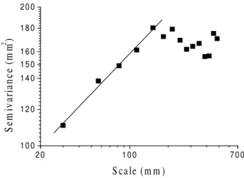
Fig. 2.An example of the relationship between the structural func-tionγ (h)plotted on a log-log diagram and the scale.
3.1.1 Fractal parameters: fractal dimension and crossover length
The main results of fractal analysis during maize and oats growth periods are listed in Tables 3 and 4, respectively. These include: sampling date, cumulative rainfall, fractal di-mension and its standard error, crossover length and its stan-dard error, coefficients of determination, upper cutoff of the straight line portion of the semivariogram plotted on a log-log scale and number of data points in this first segment of the semivariogram.
The first portion of the structural functionγ (h), when plot-ted on a log-log diagram, showed a similar trend in the 36 data sets studied, indicating the existence of a correlation be-tween semivariance and scale at small scale intervals. An example is shown in Fig. 2. The graphed results show a straight-line portion of the semivariogram at short lag dis-tances with a step slope and then a second portion, which could be approximately modelled by a horizontal sill, so that in this segment correlation between the structural function and distance in general is absent.
A self-affine model may quantify the first straight-line por-tion of the semivariogram. Thus, stable estimates of fractal parameters, D andl, could be obtained only from the first segment of the structural functions, γ (h), before the scale breaks in slope. This break in scale is mainly related with the size of the structural units, aggregates or clods, at the soil surface, consistent with previous work on soil surfaces recorded by pinmeter (Miranda, 2000; Vidal V´azquez et al., 2005, 2006) and by laser scanning (Huang and Bradford, 1992; Eltz and Norton, 1997; Davis and Hall, 1999; Vidal V´azquez et al., 2005).
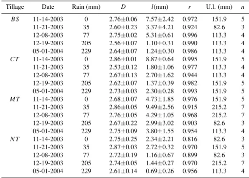
Table 3.Sampling date, cumulative rainfall, fractal parameters (Dandl)with respective standard errors (S.E.), coefficients of determination (r), upper limit of self-affine behaviour (U.l.) and number of data couples for fitting the first straight line portion of the semivariogram (n) during the maize season for different tillage treatments. (BS=bare soil,CT=conservation tillage,MT=minimum tillage,N T=no-tillage).
Tillage Date Rain (mm) D l(mm) r U.l. (mm) n
BS 11-14-2003 0 2.76±0.06 7.57±2.42 0.972 151.9 5
11-21-2003 35 2.60±0.23 3.37±4.21 0.924 82.6 3 12-08-2003 77 2.75±0.02 5.31±0.61 0.996 113.3 4 12-19-2003 205 2.56±0.07 1.10±0.31 0.990 113.3 4 05-01-2004 229 2.64±0.07 1.24±0.30 0.986 113.3 4
CT 11-14-2003 0 2.86±0.01 8.87±0.64 0.995 151.9 5
11-21-2003 35 2.53±0.12 1.80±1.06 0.977 113.3 4 12-08-2003 77 2.67±0.13 2.70±1.62 0.944 113.3 4 12-19-2003 205 2.62±0.07 1.37±0.39 0.982 151.9 5 05-01-2004 229 2.73±0.03 2.30±0.28 0.993 151.9 5
MT 11-14-2003 0 2.68±0.07 4.73±1.85 0.976 151.9 5
11-21-2003 35 2.86±0.05 9.49±2.56 0.915 215.2 7 12-08-2003 77 2.76±0.05 4.29±1.05 0.968 215.2 7 12-19-2003 205 2.67±0.22 2.99±3.02 0.903 82.6 3 05-01-2004 229 2.75±0.09 3.80±1.55 0.954 113.3 4
N T 11-14-2003 0 2.75±0.25 2.34±2.21 0.816 82.6 3
11-21-2003 35 2.87±0.03 2.72±0.32 0.970 151.9 5 12-08-2003 77 2.72±0.19 1.16±0.67 0.899 82.6 3 12-19-2003 205 2.74±0.05 1.44±0.27 0.970 215.2 7 05-01-2004 229 2.61±0.14 0.69±0.26 0.956 113.3 4
used. In our case study the lower cutoff limits of self-affinity were about the same magnitude as the distance between the pinmeter needles, i.e. 30 and 20 mm for data sets acquired during maize and oats seasons, respectively. The upper cutoff limits varied between 82.6 mm and 215.2 mm in the maize season and between 82.6 mm and 151.8 mm in the oats sea-son (Tables 3 and 4). The upper limits in this study were similar to those of a previous case study, where the semivar-iogram algorithm was applied (Vidal V´azquez et al., 2007). However, the upper cutoff limits were lower than those previ-ously estimated with the root-mean-square (RMS) algorithm (Vidal V´azquez et al., 2006, 2007).
Because the distance at which scales break, when theγ (h) structural function is used, approximately matches the char-acteristic size of the larger clods, residue fragments or in general structural elements on the soil surface, this distance has also been regarded as a fractal parameter of considerable interest. This scale has been referred to as the correlation length (Vidal V´azquez et al., 2006).
In general, linear relations between structural function and scale covering at least two orders of magnitude are required for estimating the fractal dimension,D, with low standard error values (Miranda, 2000). But in our study cases, as be-fore quoted, the range of self-affinity was between a lower cutoff of about 20 to 30 mm and an upper cutoff of about 82.6 to 215.2 mm. A millimetric grid resolution acquired by laser scanning would enhance the straight line portion of the
semivariogram on a log-log plot against the scale (Miranda, 2000; Vidal V´azquez et al., 2005). Furthermore, in each of the 36 surfaces studied, the ratio (l2/ l1)between the upper
(l2)and lower (l1)cutoffs of the structural function, γ (h),
largely exceeds 21/D, which is the minimal condition to ac-cept an experimental D value over a range of fractal self-affinity (Pfeifer and Obert, 1989).
J. Paz-Ferreiro et al.: Microrelief fractal parameters 583
Table 4.Sampling date, cumulative rainfall, fractal parameters (Dandl)with respective standard errors (S.E.), coefficients of determination (r), upper limit of self-affine behaviour (U.l.) and number of data couples for fitting the first straight line portion of the semivariogram (n) during the oats season for different tillage treatments. (BS=bare soil,CT=conservation tillage,MT=minimum tillage,N T=no-tillage).
Tillage Date Rain (mm) D l(mm) r U.l. (mm) n
BS 08-18-2004 0 2.83±0.09 11.59±6.12 0.921 82.6 3
08-31-2004 50 2.95±0.08 10.78±4.32 0.542 82.6 3 09-17-2004 153 2.98±0.02 8.73±0.90 0.559 82.6 3 10-05-2004 350 2.55±0.09 0.44±0.10 0.978 151.8 5
CT 18-08-2004 0 2.76±0.11 3.64±1.90 0.914 113.3 4
08-31-2004 50 2.79±0.15 3.43±2.11 0.891 82.6 3 09-17-2004 153 2.75±0.13 3.45±2.07 0.903 113.3 4 10-05-2004 350 2.77±0.19 2.53±1.88 0.845 82.6 3
MT 08-18-2004 0 2.86±0.07 5.49±1.78 0.877 151.8 5
08-31-2004 50 2.81±0.06 5.22±1.65 0.951 113.3 4 09-17-2004 153 2.79±0.09 4.53±1.88 0.930 113.3 4 10-05-2004 350 2.73±0.11 1.69±0.67 0.953 82.6 3
N T 08-18-2004 0 2.77±0.22 7.73±8.98 0.823 82.6 3
08-31-2004 50 2.74±0.26 7.34±10.44 0.801 82.6 3 09-17-2004 153 2.88±0.15 9.47±6.92 0.736 82.6 3 10-05-2004 350 2.81±0.11 8.27±4.85 0.876 113.3 4
estimated. Indeed, the available couple of data for fitting the power law in the first straight line part of theγ (h)structural function increased when data sets measured by non-contact laser scanning with a resolution in the order of millimeters were available (Miranda, 2000; Vidal V´azquez, 2005).
Standard errors of fractal dimension and crossover length calculated by the semivariogram method are also listed in Ta-bles 3 and 4 for data sets acquired during the maize and oats seasons, respectively. Standard errors in estimatingDvaried between 0.02 and 0.25 under maize and between 0.02 and 0.26 under oats. Standard errors in estimatinglranged from 0.26 mm to 4.21 mm and from 0.10 mm to 10.44 mm under maize and oats, respectively. Therefore, standard errors in crossover length may be as high as its estimated values, or even higher. Vidal V´azquez et al. (2006) analyzed data sets recorded by pinmeter with a comparable small size, i.e. 225 height readings per plot, using the RMS algorithm, and found D standard errors being in the range from 0.008 to 0.023 andl standard errors being in the range from 0.006 mm to 1.040 mm. These results indicate that the RMS algorithm re-duces errors in fractal parameters estimation when compared with the semivariogram algorithm by a factor of the order of one magnitude. Consequently, the use of square sampling grids instead of rectangular ones is recommended for data sets with a small number of data points, as those recorded by pinmeter.
Coefficients of determination for the straight-line portion of theγ (h)structural function were between 0.816 and 0.996 and between 0.542 and 0.978 for data sets acquired dur-ing the maize and oats seasons (Tables 3 and 4), respec-tively. The results obtained with the RMS algorithm, from
225 height readings, by Vidal V´azquez et al. (2006) were more precise, as the respective coefficient of determination varied between 0.972 and 1.000.
Fractal dimension values ranged from 2.53 to 2.87 and from 2.55 to 2.98 in the maize and oats seasons, respectively. Therefore, the 36-microrelief data sets studied showed anti-persistent features (D>2.5), also in accordance with previ-ous results of fractal parameters estimated in random mi-crorelief data sets, obtained after correction for slope and tillage marks (Miranda, 2000; Vidal V´azquez et al., 2005, 2006, 2007).
The crossover length values estimated by theγ (h) struc-tural function varied from 0.69 mm to 9.49 mm and from 0.44 mm to 11.59 mm under maize and oats, respectively. The magnitude ofl values is also consistent with previous works on data sets acquired under field conditions (Vidal V´azquez et al., 2005, 2006, 2007). These results clearly indicate a larger variation in scale of the crossover length, when compared with the fractal dimension as maximum dif-ferences between experimental data sets of this later frac-tal parameter were of 0.31 units and 0.40 units under maize and oats, respectively. Therefore, values of crossover length show a much greater sensitivity to changes in microrelief than the fractal dimension. This reinforces the relevance of the crossover length parameter as a discriminator of vertical differences in roughness.
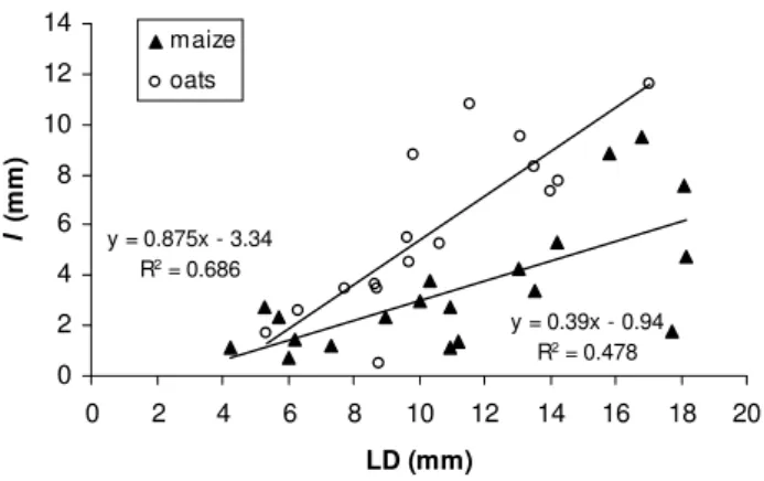
y = 0.875x - 3.34 R2 = 0.686
y = 0.39x - 0.94 R2 = 0.478 0
2 4 6 8 10 12 14
0 2 4 6 8 10 12 14 16 18 20
LD (mm)
l (mm
)
maize
oats
Fig. 3. Crossover length (l) versus limiting difference (LD) as recorded during maize and oats seasons.
(Huang and Bradford, 1992). In quantifying soil surface roughness, the fractal dimension,D, can be taken as a rela-tive measure of the spatial distribution of different size struc-tural elements on the soil surface (Huang, 1998). However fractal dimension,D, does not provide information on rough-ness vertical component. Therefore, the fractal dimension as a descriptor of horizontal variations of soil roughness should be used together with an additional index describing differ-ences in roughness height for a thorough evaluation of soil microtopography (Huang, 1998; Vidal V´azquez et al., 2006). The fractal parameter crossover length,l, and the geosta-tistical index limiting difference,LD, were compared, be-cause both indices are thought to stand for the vertical com-ponent of soil surface roughness (Eltz and Norton, 1997; Huang, 1998). Figure 3 shows the relationship betweenl andLD. Correlation coefficients were 0.478 and 0.686 for the 20 data sets acquired in the maize season and the 16 data sets acquired in the oats season, respectively (P <0.05).
Again,LDdefines the vertical component of soil rough-ness based on mean absolute elevation differences at rela-tively large distances by the sill of the first-order variance. However, l represents the intersect of the γ (h) structural function with the y-axis on a log-log scale. Therefore, the crossover length parameter is rather a measure of nugget ef-fect or discontinuity at small distances, differing from the sill or variance, which gives vertical fluctuation statistics. In fact, the magnitude of the discontinuity at small distances depends on the vertical statistics, but it may depend also on the horizontal variation of soil roughness. The relationship betweenl andLD in Fig. 3 was distinct in the maize and oats seasons, pointing to differences in surface configuration between these two experimental periods.
Crossover length and fractal dimension values estimated during the two successive growth periods showed a signif-icant correlation (P <0.05), as shown in Fig. 4. Therefore, theDvalue showed a trend, to increase aslincreased, which is an expected result, given the dependence between these
R2 = 0.544
2.5 2.6 2.7 2.8 2.9 3.0
0 2 4 6 8 10 12 14
l (mm)
D
Maize Oats
Fig. 4.Crossover length parameter (l)versus fractal dimension (D) as recorded during maize and oats seasons.
parameters in Eq. (9). A similar relationship betweenDand l was also found in previous studies (Vidal V´azquez et al., 2006, 2007).
Moreover, during the maize season l and D were sig-nificantly correlated (P <0.05) for each of the four study treatments as the respective correlation coefficients ranged fromR2=0.71 toR2=0.81. Likewise, landDwere signif-icantly correlated (P <0.05) in three out of four treatments during the oats season, as the respective correlation coeffi-cients ranged fromR2=0.71 toR2=0.90; in this case the ex-ception was theCT treatment. So, differentDandl values were associated with different soil tillage systems. Conse-quently, the couple fractal dimension and crossover length appear to be a pertinent descriptor of soil roughness. 3.2 Tillage, crop cover and rainfall effects on soil
rough-ness decay
Overall, roughness indicesRRandLDdecreased during the growth periods of maize and oats, as a function of cumula-tive rainfall, in the tilled treatments, either left fallow,BS, or under vegetative cover,CT andMT, as shown in Tables 1 and 2. Crossover length in general also decreased with cu-mulative rain, as shown in Tables 3 and 4. However, the roughness decay during maize and oats seasons was faster in theBS treatment than in theCT andMT treatments. Fur-thermore,RR,LDandlindices, in general, were not sub-stantially affected by cumulative rain in the N T treatment under maize and oats, whose surface was protected by pre-vious crop residues. Therefore, because no changes are in-duced by rainfall in no-till systems with various quantities of crop residues, one single observation along the crop season allowed characterization of soil surface roughness.
J. Paz-Ferreiro et al.: Microrelief fractal parameters 585
y = 5E-06x2
- 0.0036x + 1
R2
= 0.926 0.0
0.2 0.4 0.6 0.8 1.0 1.2 1.4
0 50 100 150 200 250 300 350 400
C ummulative pre cipitati on (mm)
RR/RR
0
Maize Oats
y = 5E-06x2
- 0.0026x + 1
R2
= 0.487
0.0 0.2 0.4 0.6 0.8 1.0 1.2 1.4
0 50 100 150 200 250 300 350 400
C ummulative pre cipitati on (mm)
LD/LD
0
Maize Oats
y = e-0. 0082x
R2
= 0.827
0.0 0.2 0.4 0.6 0.8 1.0 1.2 1.4
0 50 100 150 200 250 300 350 400
C ummulative pre cipitati on (mm)
l/l
0
Maize Oats
Fig. 5. Random Roughness (RR), Limiting Difference (LD), and crossover length parameter (l), as a function of cumulative rainfall for bare soil conventionally tilled (BS).
values listed in Tables 1 to 4. These equations had a quadratic or an exponential negative shape depending on the index and in all cases were fitted to honor the initial value for 0 mm rain. Therefore, the fitted general equation for quadratic and exponential roughness decrease were y=ax2−bx+1 andy=exp.(−ax), respectively, where y is the proportion of roughness relative to its initial value,xis cumulative rainfall andaandbare regression parameters.
y = -9E-06x2
+ 0.0018x + 1
R2
= 0.987
y = 8E-06x2
- 0.0036x + 1
R2
= 0.882
0.0 0.2 0.4 0.6 0.8 1.0 1.2 1.4
0 50 100 150 200 250 300 350 400
C ummulative pre cipitati on (mm)
RR/RR
0
Maize Oats
y = -3E-06x2
- 0.0001x + 1
R2
= 0.271
y = 1E-05x2
- 0.0036x + 1
R2
= 0.935
0.0 0.2 0.4 0.6 0.8 1.0 1.2 1.4
0 50 100 150 200 250 300 350 400
C ummulative pre cipitati on (mm)
LD/LD
0
Maize Oats
y = e-0. 001 5x
R2
= 0.673
y = e-0. 003x
R2
= 0.893 0.0
0.4 0.8 1.2 1.6 2.0
0 50 100 150 200 250 300 350 400
C ummulative pre cipitati on (mm)
l/l
0
Maize Oats
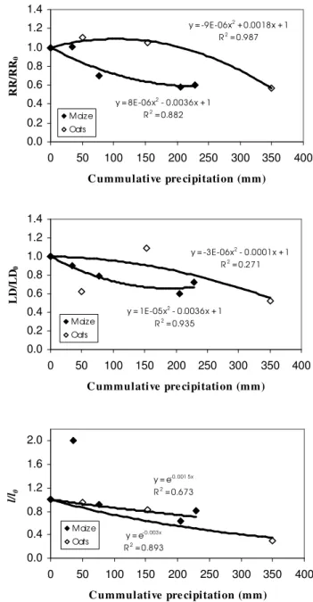
Fig. 6. Random Roughness (RR), Limiting Difference (LD) and crossover length parameter (l), as a function of cumulative rainfall, under maize and oats with conventional tillage (CT).
y = -3E-06x2
+ 0.0001x + 1
R2
= 0.592
y = 1E-05x2
- 0.0052x + 1
R2
= 0.975
0.0 0.2 0.4 0.6 0.8 1.0 1.2 1.4
0 50 100 150 200 250 300 350 400
C ummulative pre cipitati on (mm)
RR/RR
0
Maize Oats
y = -1E-05x2 + 0.0031x + 1
R2
= 0.6389
y = 7E-06x2
- 0.0037x + 1
R2
= 0.9533
0.0 0.2 0.4 0.6 0.8 1.0 1.2 1.4
0 50 100 150 200 250 300 350 400
C ummulative pre cipitati on (mm)
LD/LD
0
Maize Oats
R2
= -0.129
R2
= 0.882
0.0 0.2 0.4 0.6 0.8 1.0 1.2 1.4
0 50 100 150 200 250 300 350 400
C ummulative pre cipitati on (mm)
l/l
0
Maize
Oats
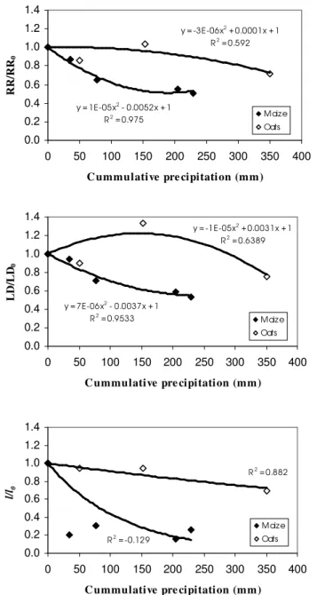
Fig. 7. Random Roughness (RR), Limiting Difference (LD), and crossover length parameter (l), as a function of cumulative rainfall, under maize and oats with minimum tillage (MT).
TheRRindex decay was best fitted by a quadratic negative relationship given byRRt/RR0=aP2−bP+1, whereRRtis random roughness for a given rainfall amount,P, andRR0
is the initial random roughness. In theBS treatment a sin-gle quadratic relationship was fitted to all the data collected in the maize and oats seasons since the relative decrease in roughness as a function of cumulative rainfall agreed for both data series. InMT andN T treatments two different relation-ships were fitted to maize and to oats data series. The fitted equations showed that underMT andN T tillage treatments, RRdecay was faster in the maize than in the oats season.
0.0 0.2 0.4 0.6 0.8 1.0 1.2 1.4
0 50 100 150 200 250 300 350 400
C ummulative pre cipitati on (mm)
RR/RR
0
Maize Oats
0.0 0.2 0.4 0.6 0.8 1.0 1.2 1.4
0 50 100 150 200 250 300 350 400
C ummulative pre cipitati on (mm)
LD/LD
0
Maize Oats
0.0 0.2 0.4 0.6 0.8 1.0 1.2 1.4
0 50 100 150 200 250 300 350 400
C ummulative pre cipitati on (mm)
l/l
0
Maize Oats
Fig. 8.Roughness indices (RRandLD), and crossover length pa-rameter (l), as a function of cumulative rainfall along the maize and oats season for no tillage (N T).
J. Paz-Ferreiro et al.: Microrelief fractal parameters 587 TheLD index decay was also best fitted by a quadratic
negative relationship. However, better correlations were ob-tained in general between cumulative precipitation andRR than between cumulative precipitation andLD. With theBS tillage treatmentLDdecay was also modelled by a single re-gression equation for the maize and oats data series. The de-cay ofLDwith theMT andN T tillage treatments, however, was modelled using two different curves. TheLD decrease was also faster in the maize than in the oats season.
Crossover length showed in general a well-defined trend, to decrease in the tilled treatments during the maize and oats seasons. In most of the rain sequences the decline of l from its initial value (0 mm rain) at the end of the season was very strong. For example, in the bare soil treatment, BS,lindex decreased 16% and 4% from initial values after 229 and 350 mm cumulative rainfall in the maize and oats seasons, respectively. However, in the maize season, MT treatment started with a relatively low value oflparameter (4.73 mm) for 0 mm rain at sowing time, which increased after 35 mm cumulative rainfall to about double the initial value (9.49 mm). This is an inconsistent result and will be discussed below. In this particular case, the value ofl for 35 mm rainfall was not taken into account for regression pur-poses.
In general, l values in the BS, CT and MT treatments exhibit a rapid decline from the initial reference state (0 mm rain) during the earlier rainfall events. The exception was again theMT treatment in the maize growth period. There-fore, l decay as a function of cumulative rainfall, P, was best fitted by a negative exponential relationship given by the equationlt/l0=exp(−aP), whereltis the crossover length for a given cumulative rainfall amount and l0 is the initial
crossover length for 0 mm rain. Crossover length was sen-sitive to differences in soil roughness conditions, allowing a description of microrelief decay due to rainfall in the tilled treatments, although better correlations between cumulative rainfall and the indicesRR andLD were most commonly obtained (Figs. 5, 6 and 7).
In a review of tillage and rainfall effects on rough-ness decay, Zobeck and Onstad (1987) described Random Roughness degradation caused by rainfall with the equation RRp=RR0exp (–0.026 P) and reported that this equation
ex-plained 76% of the variance among 418 data sets for differ-ent tillage operations and soils. Eltz and Norton (1997) con-ducted experiments with simulated rain for measuring soil surface microtopography decline using a laser scanning de-vice under fallow and soybeans. These authors found that the decrease in roughness as measured by thel index was more rapid in the earliest degradation stages than RR de-cline, after which changed very slowly. Moreover, Eltz and Norton (1987) described theRRandldecline versus kinetic energy of rain by quadratic and exponential relationships, re-spectively.
The values of the LS parameter in general were much lower at the end of the experimental period, i.e. after 229 mm rain in the maize season and 350 mm rain in the oats sea-son, than at the initial soil surfaces with 0 mm rain. This notwithstanding, in most of the rain series LS values first showed a tendency to increase and then decrease with cumu-lative rain. An increase in theLS index indicates increased slope of structural units in the soil surface. Such slope in-crease may be the result of consolidation effects during the first rain events (Eltz and Norton, 1997). TheLS decrease at the end of the growth period indicates reduction of slope at small distance intervals due to filling of small depressions around largest structural units and crust development.
There was little variation of fractal dimension with in-creasing cumulative rainfall. Small changes inDvalues ver-sus cumulative precipitation were characterized by various patterns, so that no general trend was recognized. Values for Dwere similar to those obtained in previous studies by Eltz and Norton (1997), Huang (1998) and Vidal V´azquez (2005, 2006, 2007). It is noteworthy that mean values of fractal di-mension in the maize season (2.707) were significantly lower (P <0.05) than those in the oats season (2.804), and this in spite of the fact that essentially the same tillage operations had been conducted in both periods. These differences in fractal dimension, thus, on configuration of the soil surface, may be attributed to factors such as contrasting soil water content and aggregate stability during tillage (Kamphost et al., 2000) or to plant growth effects (Mart´ınez-Turanzas et al., 1997) which further modify the soil surface configura-tion.
3.3 Physical interpretation
On agricultural soils, traditional tillage by mouldboard ploughing, followed by chisel ploughing, creates the largest degree of roughness (Kamphorst et al., 2000). Other less dominant factors influencing the configuration of soil surface microrelief may be the number of passes of the tillage tool, i.e. primary or secondary tillage, soil water content and ag-gregate stability.
even in the bare soil,BS, treatment, left fallow. Therefore, no secondary roughness increases by erosion will be taken into account.
Soil cover by plant canopy and/or cover crop and no tillage prevents soil surface from raindrop impact, reducing the rate of roughness changes. However, plant growth may increase soil surface roughness (Mart´ınez-Turanzas et al., 1997) while modifying the configuration of the soil surface microrelief, mainly due to interactions between soil surface and root sys-tem.
Again on bare soils, and when slaking is neglected, the de-cay or degree or destruction of soil roughness should depend on the initial roughness and on the kinetic energy of rain-drops. Therefore, under these conditions it may be assumed that roughness decay will follow first order kinetics, which means that the diminution of roughness per unit rain amount (or per unit kinetic energy of rain) depends on the degree of roughness that is still available. As a first approach, this can be expressed as:
Rt =R0e−kP (11)
whereRt, is the roughness at a certain time, t,R0is the initial
roughness and k is a constant describing the soil susceptibil-ity against roughness destruction.
Our results mainly support the above physical interpreta-tion. Roughness decreased with increased rain at different rates in theBS,CT andN T treatments. However, rough-ness decay did not always follow negative exponential kinet-ics. Various reasons may explain the experimental behavior of roughness decay in our case studies, which were fitted by exponential and quadratic functions, depending on the rough-ness index used (Figs. 5, 6 and 7). First, if slaking occurs, it should result in a faster roughness breakdown than can be expected from the kinetic energy alone. Second, crop and residue cover modifies the rate of decay in roughness. Also, less dominant factors such as soil water content during tillage may play a role in roughness decay dynamics. Furthermore, maize and oats root systems may modify the soil surface con-figuration, hence, the roughness decay dynamics in different ways.
In some instances, roughness indices may slightly increase with the first rainfall after roughness was increased by tillage. This initial small increase in roughness was detected for ex-ample in theCT treatment during the maize season, where the RR index increased from 14.25 to 14.40 mm for rain-falls of 0 and 35 mm, respectively (Table 1). Also, in the CT treatment during the oats season,RRandLDdetected slight roughness increases between the initial stage with 0 mm rain and the stage after 50 mm cumulative rain (Ta-ble 2). These effects have been previously reported (Eltz and Norton, 1997; Huang, 1998). Consolidation of loosened soil particles within the largest voids without significant reduc-tion in largest clods size may originate a denser soil surface with greater roughness than the freshly tilled soil surface and
also may lead to increased side slopes, as mentioned above for theLSindex.
However, the big increase in crossover length with theMT treatment in the maize season (Table 3) when the initial soil surface and the stage after 35 mm cumulative rainfall was compared was more difficult to interpret. For a cumulative rain of 35 mm, the ratiol/l0can be considered as an outlier,
because of the relative high value of the numerator. Then, the value ofl0in the freshly tilled soil surface may have been
underestimated, which would change the shape of the regres-sion betweenl/l0and cumulative rainfall.
A major problem of the characterization of roughness in our study was the small size of data sets acquired with low technology devices. The randomization process of locat-ing successive small measurement plots for characterizlocat-ing a given treatment may partly explain the dispersion of the regression functions developed for roughness decay. This notwithstanding, our microrelief data sets have been found to be self-affine in a small range of scales with an upper limit matching the size of the largest structural units in the soil surface and a lower limit equal to the horizontal resolution of point heights measurements. Therefore, accuracy and re-producibility of the roughness indices and fractal parameters could be increased in different ways: i) a large measuring grid could be used and a higher number of readings could be taken, ii) replicate microplots could be measured on each plot and on each date, and iii) the same microplot on each treatment could be used on each date.
The fractal parametersD andl have been useful to fur-ther quantifying the soil surface configuration and to discrim-inate between soil uses and crop cover. MeanDvalues were higher in the oats season, which means a more rugged soil surface, even if parameters accounting for vertical roughness, RRandLD, did not follow this trend. Also, the relationships betweenRRandLDversuslin the maize and the oats pe-riods were not equivalent (see Fig. 3), which is indicative of differences in soil surface configuration properties between the two crop canopies.
4 Conclusions
Microrelief measurements taken on small plots and consist-ing of 225 height measurements showed spatial correlation after slope and tillage trend removal in a limited range of scales, allowing to estimate two fractal indices, fractal di-mension and crossover length.
J. Paz-Ferreiro et al.: Microrelief fractal parameters 589 Both random roughness and limiting difference decreased
from initial values in a similar proportion with increasing rainfall. Crossover length index,exhibited a faster decrease from the initial values than random roughness and limiting difference. Even thought there was little variation in fractal dimension with cumulative rainfall this parameter was found to be significantly higher in the oats than in the maize season.
Acknowledgements. This work was partially funded by MEC
(Spain) under research project CGL2005 – 08219 – C02-01 – HID. The authors are grateful to three anonymous referees for providing valuable comments.
Edited by: A. Tarquis
Reviewed by: three anonymous referees
References
Allmaras, R. R., Burwell, R. E., Larson, W. E., and Holt, R. F.: Total porosity and random roughness of the interrow zone as in-fluenced by tillage, USDA Conservation Res. Rep., 7, 22 pp., 1966.
Armstrong, A. C.: On the fractal dimensions of some transient soil properties, J. of Soil Sci., 37, 641–652, 1986.
Bertol, I., Schick, J., Batistela, O., Leite, D., Visentin, D., and Cogo, N. P.: Erosividade das chuvas e sua distribuic¸˜ao entre 1989 e 1998 no Municipio de Lages (SC) (In portuguese), Brazilian Re-vue of Soil Science, 26, 455–464, 2002a.
Bertol, I., Schick, J., Batistela, O., Leite, D., and Amaral, A. J.: Erodibilidade de um Cambissolo H´umico alum´ınico l´eptico, de-terminada sob chuva natural entre 1989 e 1998 em Lages (SC) (In portuguese), Brazilian Revue of Soil Science, 26, 465–471, 2002b.
Bertol, I., Amaral, A., Vidal V´azquez E., Paz Gonz´alez, A., Bar-bosa, F. T., and Brignoni, L. F.: Relac¸˜oes da rugosidade super-ficial do solo com o volume de chuvas e com a estabilidade dos agregados em ´agua (In Portuguese), Brazilian Revue of Soil Sci-ence, 30, 543–555, 2006.
Bertuzzi, P., Rauws, G., and Courault, D.: Testing roughness in-dices to estimate soil surface changes due to simulated rainfall, Soil Till. Res., 17, 87–99, 1990.
Burrough, P. A.: Multiscale sources of spatial variation in soil. I. The application of fractal concepts to nested levels of soil varia-tion, J. Soil Sci., 34, 577–597, 1983a.
Burrough, P. A.: Multiscale sources of spatial variation in soil. II. A non-Brownian fractal model and its application in soil survey, J. Soil Sci., 34, 599–620, 1983b.
Carr, A. D. and Benzer, W. B.: On the practice of estimating fractal dimension, Math. Geol., 23, 945–958, 1991.
Currence, H. D. and Lovely, W. G.: The analysis of soil surface roughness, Trans. ASAE, 13, 710–714, 1970.
Darboux, F. and Huang, C. H.: Does soil surface roughness increase or decrease water and particle transfer?, Soil Sci. Soc. Am. J., 69, 748–756, 2005.
Davies, S. and Hall, P.: Fractal analysis of surface roughness by using spatial data, Journal of the Royal Statistical Society (Series B), Statistical Methodology, 61, 3–37, 1999.
Dexter, A. R.: Effect of rainfall on the surface micro-relief of tilled soil. J. Terramechanics, 14, 11–22, 1977.
Eltz F. L. F. and Norton L. D.: Surface roughness changes as af-fected by rainfall erosivity, tillage, and canopy cover, Soil Sci. Soc. Am. J., 61, 1746–1755, 1997.
Favis-Mortlock, D. T., Boardman, J., Parsons, A. J., and Lascelles, B.: Emergence and erosion: a model for rill erosion and devel-opment, Hydrol. Processes, 14, 2173–2205, 2000.
Gallart, F. and Pardini, G.: Perfilru: un programa para el an´alisis de perfiles microtopogr´aficos mediante el estudio de la geometr´ıa fractal, (in Spanish), Cadernos Lab. Xeol´oxico de Laxe 21, 169– 178, 1996.
Hairsine, P. B., Moran, C. J. and Rose, C. W.: Recent developments regarding the influence of soil surface characteristics on overland flow and erosion. Aus. J. Soil. Res., 30, 249–264, 1992. Hansen, B., Sch¨onning, P., and Sibbesen, E.: Roughness indices for
estimation of depression storage capacity of tilled soil surfaces, Soil and Tillage Research, 52, 103–111, 1999.
Helming, K., R¨omkens, M. J. M., and Prasad, S. N.: Surface rough-ness related processes of runoff and soil loss: a flume study, Soil Sci. Soc. Am. J., 62, 243–250. 1998.
Huang, C. and Bradford J. M.: Depressional storage for Markov-Gaussian surfaces, Water Resour. Res., 26, 2235–2242, 1990. Huang, C. and Bradford J. M.: Applications of a laser scanner to
quantify soil microtopography, Soil Sci. Soc. Am. J., 56, 14–21, 1992.
Huang, C.: Quantification of soil microtopography and surface roughness, in: Fractals in Soil, edited by: Baveye, P., Parlange, J. Y. and Stewart, B. A., Science, 377 pp., 1998.
Kamphorst, E. C., Jetten, V., Guerif, J., Pitkanen, J., Iversen, B. V., Douglas, J. T., and Paz, A.: How to predict maximum water storage in depressions from soil roughness measurements, Soil Sci. Soc. Am. J., 64, 1749–1758, 2000.
Linden D. R. and van Doren, D. M.: Parameters for characterizating tillage induced soil surface roughness, Soil Sci. Soc. Am. J., 50, 1560–1565, 1986.
Lovejoy, S. and Schertzer, D.: Scaling and multiftractal fields in the solid earth and topography, Nonlin. Processes Geophys., 14, 465–502, 2007
Malinverno, A.: A single method to estimate the fractal dimension of self-affine series, Geophysical Research Letters, 17(11), 1953, 1990.
Mandelbrot, B. B.: The fractal geometry of nature, Freeman, San Francisco, 1983.
Mandelbrot, B. B.: Self-affine fractals and fractal dimension, Phys-ica Scripta, 32, 257–260, 1985.
Mandelbrot, B. B. and van Ness, J. V.: Fractal Brownian motions, fractal noises and applications, SIAM Review, 10(4), 422–437, 1968.
Martinez-Turanzas, G. A., Coffin, D. P., and Burke, I. C.: Devel-opment of microtopography in a semi-arid grassland: Effects of disturbance size and soil texture. Plant and Soil, 161, 163–171, 1997.
Merril, S. D., Huang, C., Zobeck, T. M., and Tanaka, D. L.: Use of the chain set for scale-sensitive and erosion-relevant measure-ments of soil surface roughness, in: Sustaining the global farm, edited by: Stott, D. E., Mothar R. H., and Steihardt, D. C., 594– 600, 2001.
Pardini, G.: Fractal scaling of surface roughness in artificially weathered smectite-rich soil regoliths, Geoderma, 117(11), 157– 167, 2003.
Pardini, G. and Gallart, F.A.: Combination of laser technology and fractals to analyse soil surface roughness, Eur. J. Soil Sci., 49, 197–202, 1998.
Pfeifer, P. and Obert, M.: Fractals: basic concepts and terminology, in: The fractal approach to Heterogeneous Chemistry, edited by: Avnir, D., Surfaces, Colloids, Polymers. Wiley. New York, 11– 43, 1989.
R¨omkens, M. J. M. and Wang, J. Y.: Effect of tillage on surface roughness, Trans. ASAE 29, 429–433, 1986.
Soil Survey Staff Division: Soil survey manual, USDA Handb. 18. US Gov. Print. Office. Washington DC, 1993.
Vidal V´azquez, E., Paz Gonz´alez, A., and Vivas Miranda, J. G. V.: Characterizing isotropy and heterogeneity of soil surface mi-crotopography using fractal models, Ecological Modelling, 182, 337–353, 2005.
Vidal V´azquez, E., Miranda, J. G. V., Alves, M. C., and Paz Gonz´alez, A.: Effect of tillage on fractal indices describing soil surface microrelief of a Brazilian Alfisol, Geoderma, 134(3–4), 428–439, 2006.
Vidal V´azquez, E., Miranda, J. G. V., and Paz Gonz´alez, A: De-scribing soil surface microrelief by crossover length and fractal dimension, Nonlin. Processes Geophys., 14, 223–235, 2007, http://www.nonlin-processes-geophys.net/14/223/2007/. Voss, R. F.: Random fractals: characterization and measurement.
Scaled Phenomena in Disordered Systems. New York. Plenum Press. 1-11, 1985.
Wagner, L. E. and Yiming Yu: Digitization of profile meter pho-tographs. Trans. Am. Soc. Agric. Eng., 34, 412–416, 1991. Zobeck, T. M. and Onstad, C. A.: Tillage and rainfall effects on
random roughness: A review. Soil and Tillage Research, 9, 1– 20, 1987.