Credit Scoring Using Genetic Programming

NOVA

IMS

Credit Scoring Using Genetic Programming

David Micha Horn

Advisor: Professor Leonardo Vanneschi

Internship report

presented as partial requirement for

NOVA Information Management School

Instituto Superior de Estatística e Gestão de Informação

Universidade Nova de Lisboa

CREDIT SCORING USING GENETIC PROGRAMMING

by

David Micha Horn

Internship report presented as partial requirement for obtaining the Master’s degree in Advanced

Analytics.

Advisor:Leonardo Vanneschi

ACKNOWLEDGEMENTS

“I am not going to thank anybody, because I did it all on my own”

—Spike Milligan, on receiving the British Comedy Award for Lifetime Achievement

I would like to thank my advisor Professor Leonardo Vanneschi who sparked my interest in Genetic Programming and gave me important remarks on the thesis.

Furthermore, I would like to express my gratitude to Dr. Klaus-Peter Huber who gave me the opportunity to do an internship and write my thesis with Arvato Financial Solutions.

My thank also goes to my advisor Sven Wessendorf for giving me guidance and the very necessary suggestions for improvements in this thesis.

Special thanks to Dr. Karla Schiller for introducing and explaining the process of credit scoring to me. Additionally, I would like to thank her and Dr. Markus Höchststötter for letting me take part in their project, and thus providing me with a topic for this thesis.

I gratefully acknowledge the support given by Achim Krauß and Hannes Klein towards my understanding of the data used in this thesis as well as Isabell Schmitt whose knowledge of administrative mechanisms and resources within Arvato Financial Solutions proved extremely beneficial for my work.

ABSTRACT

Growing numbers in e-commerce orders lead to an increase in risk management to prevent default in payment. Default in payment is the failure of a customer to settle a bill within 90 days upon receipt. Frequently, credit scoring is employed to identify customers’ default probability. Credit scoring has been widely studied and many different methods in different fields of research have been proposed.

The primary aim of this work is to develop a credit scoring model as a replacement for the pre risk check of the e-commerce risk management system risk solution services (rss). The pre risk check uses data of the order pro-cess and includes exclusion rules and a generic credit scoring model. The new model is supposed to work as a replacement for the whole pre risk check and has to be able to work in solitary and in unison with the rss main risk check.

An application of Genetic Programming to credit scoring is presented. The model is developed on a real world data set provided by Arvato Financial Solutions. The data set contains order requests processed by rss. Results show that Genetic Programming outperforms the generic credit scoring model of the pre risk check in both clas-sification accuracy and profit. Compared with Logistic Regression, Support Vector Machines and Boosted Trees, Genetic Programming achieved a similar classificatory accuracy. Furthermore, the Genetic Programming model can be used in combination with the rss main risk check in order to create a model with higher discriminatory power than its individual models.

KEYWORDS

INDEX

List of Figures iv

List of Tables v

1 Introduction 1

2 Theoretical Framework 4

3 risk solution service 10

4 Research Methodology 14

4.1 Dataset . . . 17

4.2 Genetic Programming . . . 21

4.2.1 Initialization . . . 22

4.2.2 Evaluation Criteria . . . 23

4.2.3 Selection . . . 25

4.2.4 Genetic Operators . . . 26

4.3 Applying Genetic Programming . . . 28

4.4 Calibration . . . 31

5 Results 34 5.1 Discriminatory Power of GP and Comparison to other Classifier . . . 35

5.2 Discriminatory Power of GP in Collaboration with the Credit Agency Score . . . 38

5.2.1 Varying Threshold . . . 38

5.2.2 Fixed Threshold . . . 40

6 Conclusion and Discussion 43

7 Limitations and Recommendations for Future Works 45

8 References 47

LIST OF FIGURES

1 Relationship between Default Probability and Scores . . . 4

2 Example distributions of goods and bads . . . 4

3 rss System . . . 10

4 rss Risk Management Services . . . 11

5 Risk Check . . . 11

6 Prescore Behavior in Score Range . . . 12

7 Prescore Distribution of Goods and Bads . . . 13

8 Overall Work Flow . . . 16

9 Discretization Plot . . . 20

10 Example Syntax Tree . . . 21

11 GP Process . . . 22

12 Confusion Matrix . . . 23

13 Example ROC curve . . . 24

14 Genetic Operators . . . 27

15 Median Fitness over all Runs . . . 28

16 Model with highest Fitness Value . . . 30

17 Calibration Plots . . . 32

18 GP Distribution . . . 35

19 ROC curve and PR diagram . . . 36

20 Score Distribution of ABIC and GP . . . 38

LIST OF TABLES

1 Discretization of Continuous Variables . . . 18

2 Input Variables . . . 19

3 GP Parameter Settings . . . 21

4 Occurrences of Variables . . . 29

5 Effect of IR on GP, SVM and BT . . . 36

6 Classifier Accuracies . . . 40

7 GP Order Value Comparison . . . 41

1.

INTRODUCTION

E-commerce vendors in Germany have to deal with a peculiarity. Commonly used payment types like credit cards or PayPal represent a relatively low market share and the majority of orders are processed using open invoice instead. Using open invoice, a vendor bills his customers for goods and services only after delivery of the product. Thus, the vendor grants his customer a credit to the extend of the invoice. Usually, the vendor sends his customers an invoice statement as soon as the products are delivered or provided. The invoice contains a detailed statement of the transaction. Because the customer receives his purchase before payment, it is called ’open’ and once the payment is received the invoice is closed. Around 28% of customers in Germany choose open invoice as payment type, a market share that comes with reservations for the vendors (Frigge, 2016). Customers are used to pay using open invoice in an ex-tend that it is a payment type selection requirement. Incidentally, around 30% of customers who abort the purchasing process do so because their desired payment type is unavailable and 68% of customers name open invoice the most desired payment type next to the ones already available (Fittkau & Maaß Consulting, 2014; Wach, 2011). However, open invoice is most prone to payment disruptions. Among the most common reasons vendors find that customers simply forget to settle the bill or delay the pay-ment on purpose but around 53% of vendors named insolvency as one of the most common reasons for payment disruption (Weinfurner et al., 2011). The majority of cases that conclude in default on payment are assigned to orders with open invoice as payment type, with more than 8% of all orders defaulting (Seidenschwarz et al., 2014). E-commerce vendors find themselves in a conflict - offering open invoice decreases the order abortion rate but increases the default on payment rate. The former has a positive effect on revenue while the latter drives it down. Additionally, default on payment has a negative impact on the profit margin, due to costs arising through provision of services and advance payments to third parties. In order to break through this vicious circle vendors can fall back on a plethora of methods. Many tackle this conflict by implementing exclusion rules for customer groups they consider especially default-prone, for instance customers who are unknown to the vendor or whose order values are con-spicuously high. Another approach, used by more than 30% of e-Commerce vendors in Germany, is to fall back on external risk management services (Weinfurner et al., 2011).

Risk management applications aim at detecting customers with a high risk of defaulting. Those appli-cations are frequently build using credit scoring models. Credit Scoring analyzes historical data in order to isolate meaningful characteristics that are used to predict the probability of default (Mester, 1997). However, the probability of default is not an attribute of potential customers but merely a vendors’ assessment if the potential customer is a risk worth taking. Over the years, credit scoring has evolved from a vendors’ gut decision over subjective decision rules to a method based on statistically sound models (Thomas et al., 2002).

risk check and a main risk check in order to satisfy different demands in an international environment. The main risk check is based on a credit agency score that uses country specific solvency information on individuals. Hence, the main risk check is inoperable in countries without accessible solvency infor-mation. Contrarily, the pre risk check was designed to be always operable and to ensure that the risk check returns an evaluation of the customers’ default probability. For this purpose, the pre risk check uses data transmitted by the customer during the order process. However, the pre risk check is based on a generic model without statistical sound backup. In this work Genetic Programming is used to build a credit scoring model to replace the existing rss pre risk check.

Proposed by Koza (1992), Genetic Programming is an evolutionary computation method in the research area of optimization that searches for a solution in a search space. For this purpose a population of potential solutions is created and then submitted to an optimization process that makes use of the idea of survival of the fittest. Inspired by Darwin’s theory about evolution, Genetic Programming employs evolutionary mechanisms such as inheritance, selection, crossover and mutation in order to gradually evolve new solutions to a problem. In a credit scoring environment, Genetic Programming initializes a population of discriminant functions in order to classify customers into bads and goods. This population is subsequently submitted to the genetic operators to find the best discriminant function.

Marques et al. (2013) state five major characteristics of computational intelligence systems such as evo-lutionary computation that are especially appealing in credit scoring:

• Learning • Adaption • Flexibility • Transparency • Discovery

The first characteristic, learning, describes the ability to learn decisions and tasks from historical data. Adaption represents the capability to adapt to a changing environment. Hence, there is no restriction to specific situations or economic conditions. The flexibility of computational intelligence systems al-lows for utilization even with incomplete or unreliable data sets. Furthermore, Marques et al. (2013) describe computational intelligence systems to be transparent, is a sense that resulting decisions are explainable. The outputs may be revisable in general, but for example Goldberg (1989) criticizes the poor comprehensibility of Genetic Algorithms which can be transfered to Genetic Programming. Taking into account that Marques et al. (2013) point out the potential importance to provide explanations of how decisions have been made due to legal reasons, transparency as characteristic has to be called into question. Lastly, discovery represents the ability to discover previously unknown relationships.

Research repeatedly showed the benefits of Genetic Programming and its utility in Credit Scoring. How-ever, credit scoring is usually employed using data from the financial sector and other sectors are rarely considered. While credit scoring was originally implemented by mail-order companies, it is unclear if benefits remain present but underutilized. Hence, the motivation and aim of this work is to extend current research in credit scoring by employing Genetic Programming on a data set that contains orders from e-commerce vendors, a field that has so far been neglected.

2.

THEORETICAL FRAMEWORK

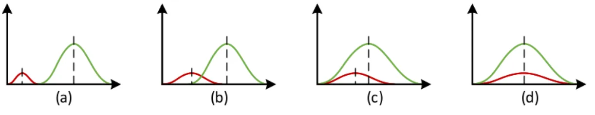
Credit Scoring is a widely used application by financial institutions for the determination of applicants default probability and the subsequent classification into a good applicant group (the ”goods”) or a bad applicant group (the ”bads”) (Thomas et al., 2002). Consequentially, applicants are rejected or accepted as customers based on the classification. Credit scoring represents a binary classification problem that enables the usage of methods that deal with binary response data (Henley, 1995). To evaluate the credit risk of loan applications, Credit Scoring targets at isolating effects of applicants’ characteristics on their default probability. The default probability is mapped to a numerical expression – the score – that in-dicates the creditworthiness of the applicant and enables the creditor to rank order applicants. The relationship between default probability and scores is depicted in figure 1. The mean scores over all

B

a

d

R

a

te

Scores

Figure 1: Relationship between Default Probability and Scores

applicants who perform well should be higher than the mean scores over all applicants who perform badly. The better the mean scores separate good and bad applicants, the higher the discriminatory power of the model (Mester, 1997). Figure 2 shows the distributions of bads and goods for four ex-ample models, with the scores on the x-axis and the number of observations on the y-axis. The bads are represented by the red line, whereas the goods are represented by the green line. The dashed line depicts the mean values for bads and goods. In model (a) bads and goods are non-overlapping, and hence the model has maximum discriminatory power. Model (b) shows slightly overlapping goods and bads. Thus, the discriminatory power is reduced compared to the maximum, but still on a high level. In model (c) goods and bads are heavily overlapping which implies low discriminatory power. Finally, the mean scores of goods and bads in model (d) are identical, and hence the model incorporates no discrim-inatory power. The classification and hereupon decision if an applicant is being rejected or accepted is

(a) (b) (c) (d)

Figure 2: Example distributions of goods and bads

into account risk characteristics of rejected applications. Models build solely on data about accepted applications should only be used to assess the probability of default for a similar population of accepted requests and thus contradicting the problem specifications of credit scoring. In order to decrease the bias in data, an approach called ”reject inference” is often times employed. Reject Inference targets at inferring the true status of rejected applications (Thomas, 2000; Henley, 1995).

The benefits of a credit scoring model for financial institutions are threefold. First, the application of a credit scoring model reduces the time needed for the approval process. The possible time savings vary depending on how strictly the proposed cut-off threshold is followed. If the threshold is followed strictly, credit applicants above or below the threshold are automatically accepted or rejected. Contrariwise, if the threshold is not followed strictly, the applications within a certain range around the threshold can be reevaluated. In either case the efficiency of credit scoring can improve greatly because applicants far away from the threshold are automatically detected and categorized. Second, because applying and handling the application takes less time, both parties save money. Third and lastly, both creditor and applicant benefit from an increased objectivity in the loan approval process. Using a credit score model ensures that the same criteria are applied to all applicants regardless of the personal feelings from the creditor’s person in charge towards the applicant. Additionally, the creditor gains the capability to doc-ument factors with a disproportionally negative effect on certain groups of applicants (Mester, 1997). The objectives in credit scoring for mail-order and e-commerce vendors differ from finance and banking. Rejected individuals are not denied from purchasing goods but restricted to secure payment methods at point of sale. Secure payment methods require the customer to pay the ordered goods before shipment or on delivery, e.g. advanced payment, credit card, pay on delivery or PayPal. Denying open invoice and other insecure payment methods increases the abortion rate during the payment process. Individuals retained in the payment process are usually measured by the conversion rate, i.e. the ratio of individ-uals finishing the order process to individindivid-uals entering the payment process. Hence, credit scoring in e-commerce aims at lowering default on payment by rejecting individuals with a high probability of de-fault from purchasing goods using insecure payment methods whilst retaining a maximum conversion rate.

Sackmann et al. (2011) divide the risk of default in payment into two dimensions. The first dimension is represented by individuals who are unable to settle their bills because of insolvency or illiquidity and the second dimension is represented by individuals who are unwilling to settle their bills because they engage in fraud. Using those dimensions, they define four risk categories.

1. Ability and Willingness to settle bill 2. Inability to settle bill

3. Unwillingness to settle bill

4. Inability and Unwillingness to settle bill

by impersonating others for which adequate prevention measures exists. Fraud prevention can also be integrated into credit scoring models, which covers the fourth risk category (Sackmann et al., 2011). Additionally, those approaches may have a positive effect with individuals who enter their information wrongly by accident but are both able and willing to settle their bills. Denying them from a purchase based on insecure payment methods may prompt them to review their input data and thus decrease wrong deliveries and dunning costs.

The ability to combine the identification of those who are unable and those who are unwilling to settle their bills elevates credit scoring to a very capable risk management tool in e-commerce. Incidentally, the history of credit scoring goes back to mail-order companies (the predecessor of e-commerce ven-dors) in the 1930s. Credit decisions were made on the basis of subjective judgment by credit analysts. Thus, applicants may be rejected by a credit analyst but accepted by another. In an effort to dimin-ish the respective inconsistencies mail-order companies introduced a numeric scoring system. Shortly thereafter, Durand (1941) used Fisher’s linear discriminant introduced by Fisher (1936) to differentiate between good and bad loans. Results were not utilized in a predictive setting but to extract attributes that indicate good and bad borrowers. Credit scoring was boosted with the start of World War II be-cause credit analysts were drafted into military service leading to a shortage in personnel with respective knowledge. Hence, credit analysis provided the rules of thumb they used in the credit decision process for non-experts to be used (Thomas et al., 2002).

After the war, credit scoring slowly emerged as target of scientific research. Wolbers (1949) investi-gated the effect of credit scoring in a department store chain and McGrath (1960) for an automobile dealer. Both report major decline in credit loss. Myers and Forgy (1963) developed a scoring system to replace a numerical scoring system based on pooled judgment of credit analysts. Although they noted that their scoring system was adopted they do not offer a comparison with the existing system but only between different systems they proposed. In their conclusion they remark that they did not select the system with the highest performance due to unacceptable weights assignments. In 1956, Bill Fair and Earl Isaac founded Fair, Isaac, and Company, the first consultancy to provide a credit scoring system and nowadays known as FICO. Incidentally, FICO is the predecessor of the risk management division of AFS. The decisive milestone in the history of credit scoring was the Equal Credit Opportunity Act (ECOA) in the United States of America in 1974. Under the ECOA race, color, national origin, religion, martial status, age, sex or level of involvement in public assistance is prohibited to be used in credit scoring. Furthermore, the ECOA classifies scoring systems into those that are ”empirically derived and statisti-cally valid” and those that are not. As a result, judgmental scoring systems were weakened and scoring systems based on statistically valid models generally accepted (United States Code, 1974; Thomas et al., 2002; Mays, 2001).

that credit risk has to be quantified based on formal methods using data. Hence, it is virtually impos-sible for organizations in member countries to employ risk sensitive capital allocations without the use of credit scoring techniques (Khashman, 2010; Oreski et al., 2012; Marques et al., 2013). As a result, credit scoring attracted additional notice from scientists and lead to an increase in research. The Basel Accords only affect banking and financial organizations which directs the focus of published papers on these research areas.

Over the years a great number of different approaches to obtain a satisfactory credit scoring model have been proposed. The classical approaches involve methods such as linear discriminant models (Re-ichert et al., 1983), logistic regression (Wiginton, 1980; Henley, 1995), k-nearest neighbors (Henley and Hand, 1996) and decision trees (Davis et al., 1992), but more sophisticated approaches such as neural networks (Desai et al., 1996; Malhotra and Malhotra, 2002; West, 2000) and genetic programming (Ong et al., 2005; Abdou, 2009) have also been utilized.

One of the few papers using genetic programming for credit scoring by Ong et al. (2005) compared ar-tificial neural networks, classification and regression tree, C4.5, rough sets and logistic regression with plain genetic programming using two well known data sets, namely, credit data sets from Australia and Germany. Genetic programming was used in order to determine the correct discriminant function au-tomatically and to use the model with both big and small data sets. Comparing the error rates, the authors showed that genetic programming outperforms the other models in both data sets but noted that artificial neural networks and logistic regression also performed well. The authors concluded that GP is a non-parametric tool that is not based on any assumptions concerning the data set, which makes GP suitable for any situations and data sets. Additionally, the authors stated that GP is more flexible and accurate than the compared techniques.

Huang et al. (2007) investigated the credit scoring accuracy of three hybrid Support Vector Machines (SVM) based data mining approaches on the Australian and German data set. The SVM models were combined with the grid search approach in order to improve model parameters, the F-Score for fea-tures selection and Genetic Algorithms in order to obtain both the optimal feafea-tures and parameters automatically at the same time. The results of the hybrid SVM models are compared to other data min-ing approaches based on Artificial Neural Networks, Genetic Programmmin-ing and C4.5. The authors found that the best results were achieved by Genetic Programming, followed by their hybrid SVM approach. They pointed out that GP and their hybrid SVM approach used less features than input variables due to the automatic feature selection.

Zhang et al. (2007) apply Genetic Programming, Backpropagation Neural Networks and Support Vector Machines on credit scoring problems using the Australian and German data sets. Additionally, they con-struct a model by combining the classification results of the other models using majority voting. The accuracy is used as evaluation criteria. They show that the different models obtain good classification results but their accuracies differ little. Furthermore, the combined model shows better overall accura-cies.

cor-rectly classified cases, the estimated misclassification cost takes into account the costs that arise from different types of error. In his conclusion the author stated that the preferred model depends on which evaluation criterion is used but that the results are close.

Chen and Huang (2003) used credit scoring models based on artificial neural networks (NN) and genetic algorithms (GA) on the Australian and German data sets. The NN model was used for classification, fol-lowed by a GA-based inverse classification. The latter was implemented to gain a better understanding of the rejected instances and to reassign them to a preferable accepted class, which balances between cost and preference. They conclude that NNs are a promising method and GAs incorporates attractive features for credit scoring.

A two-stage GP model to harvest the advantages of function-based and induction-based methods is implemented by Huang et al. (2006) using the Australian and German data sets. In the first stage, GP was used to derive if-then-else rules and in the second stage, GP was used to construct a discrimina-tive function from the reduced data set. The two-stages split was implemented to restrict the model complexity and therefore ensured comprehension of the decision rules. Subsequently, only few general rules for every class were derived instead of every rule for the whole data set. The second stage derived the discriminative function for forecasting purposes. The results were compared to a number of data mining techniques but showed no significant improvement of two-stage GP over plain GP. However, the authors pointed out that additional to general GP advantages like automatic feature selection and func-tion derivafunc-tion, two-stage GP provided intelligence rules that can be independently used by a decision maker.

Fogarty (2012) argues that GAs produce results that are only slightly better than traditional techniques but have little additional utilization in the industry and are thwarted by transparency legislation and regulation. Although he briefly acknowledges advantages of GAs stated by other researchers, he fails in including those advantages into his overall assessment of GAs. Therefore, he employed Genetic Al-gorithms (GA) as a maintenance system for existing scoring systems instead of using GAs for model development. Maintaining credit scoring models becomes necessary once a shift in population leads to deterioration of the models’ discriminative capabilities. Fogartys approach included the employment of GAs on 25 models that were originally developed using logistic regression. Models and data sets were provided by a unnamed finance company. The performances of the resulting models were compared to the source models. Because legislative and regulatory constraints still hold for revised models, better or similar performing models were only marked for redevelopment. The author found that 18 models performed significantly better than their source model, compared to 4 models that performed equally good. In 3 cases did the models not perform satisfactory due to overfitting the data and no model per-formed worse than its source model. The author concluded that GAs are a useful approach as a credit scoring maintenance system.

descrip-tive fuzzy system is that in the latter fuzzy rules are associated with linguistic concepts, which makes them more intuitive, more humanly understandable and increases the comprehensibility considerably. Hoffmann et al. (2002) use data from a major Benelux financial institution and Hoffmann et al. (2007) additionally uses the publicly available Australian and German data sets as well as data about breast cancer and diabetes. The evaluation measure in both papers is the accuracy. Hoffmann et al. (2007) conclude that both approximate and descriptive fuzzy rules yield comparable results. They reason that the boosting algorithm employed compensates for weaknesses in the individual rules and hence evens out the results. Comparing their approaches with other techniques shows no clear indication of a su-perior method. Results are either indistinguishable or the susu-perior method depends on the data set. Hoffmann et al. (2007) remark an important trade-off between the fuzzy rule systems. The approximate fuzzy rules yield few rules but with low comprehensibility while the descriptive fuzzy rules yield a larger rulebase with more intuitive linguistic rules. Their works provide one of several useful approaches for the extraction of humanly readable rules that provide explanations of how decisions have been made (Goldberg, 1989). Subsequently, their approach closes the gap in the characteristics of computational intelligence systems stated by Marques et al. (2013).

3.

RISK SOLUTION SERVICE

Risk solution service (rss) is a risk management service that aims at covering the whole order process of ecommerce retailers’ customers.

Its objectives are threefold. First, increase of conversion rate and customers’ retention in the E-Shop by improving differentiation and managing of payment methods. Next, enhance cost control by providing innovative pricing models and configurable standard solutions in different service levels. Last, improve discriminatory power by combining current and historical customer information.

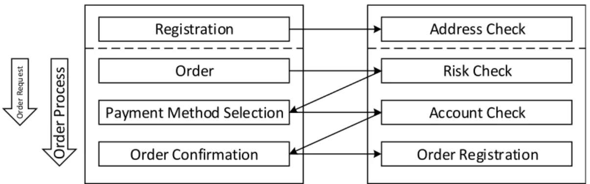
The rss system works as shown in figure 3. Customer actions are registered by the client system and passed on to the rss backend. Depending on the customer action, service calls are triggered as depicted in figure 4 and explained below. The data content of the service calls is passed on to the ASP platform that carries out the scoring of the customer. The ASP platform saves the request data on a logging database from where it is passed on to an archive and a reporting database. From the latter, the data is passed on to the data warehouse and merged with additional information from an extra rss database. The reporting system in the portal obtains the data from the data warehouse. Additionally, the client specific configuration is retained on the portal for easy access by the client. On every data transfer, the data is reduced and partly transformed. Hence, the data in the data warehouse does not entirely match the data used in the service calls.

Customer

Action Service Call

Client System rss Backend

ASP

Operational System

Configuration Portal

Reporting

Data Data

Data Data Data

Logging rss Database

Archive Temp DWH

Figure 3: rss System

1. validation of correct postal syntax

2. verification and if necessary correction of mail address

3. verification of deliverability by checking against a list of known addresses

Once the customer placed the order with the client, a risk check deploys and returns a risk assessment to the client. Based on the risk assessment, the client offers his customers selected payment methods from which the customer may choose whichever he prefers. In case the customer chooses direct debit, an account check deploys and checks the customers’ submitted account data. The account check verifies the validity of the entered account data by:

1. validation of correct syntax

2. comparison with whitelist of existing bank identification numbers

3. comparison with blacklist of publicly visible bank accounts, e.g. public institutions or charity or-ganizations

In case the customer is accepted an order confirmation is transmitted and the order gets registered in the rss system.

Registration

Order

Payment Method Selection

Order Confirmation

Address Check

Risk Check

Account Check

Order Registration

O

rd

e

r

P

ro

ce

ss

O

rd

e

r

R

e

q

u

e

st

Figure 4: rss Risk Management Services

Rss is designed to work not only with the existing scoring system AFS provides but also with scoring systems of other providers. Hence, in order to ensure operationally in absence of the AFS credit agency score, the Risk Check was split into two modules that work in combination and on its own. The risk check consists of the pre risk check and the main risk check, as depicted in figure 5. The former being a combination of a pre check and a pre score and the latter calling different credit agency scoring systems. Added together, they compose the rss score.

Risk Check

Pre Risk Check

Pre Check Pre Score

Main Risk Check

Credit Agency Score

Figure 5: Risk Check

the years. However, neither the original design nor any update was based on a statistically sound model. Instead, a generic scorecard was developed, which is generally done whenever data is unavailable. The pre risk check consists of a pre check and a pre score. The former is a combination of exclusion rules that lead to the rejection of a request if triggered or otherwise to a pass on to the pre score, which assigns a score according to the request data. The latter is centered on 0 in order to work as an “on top” addition or deduction to the credit agency score. The pre check matches requests with a blacklist, compares the request basket value to a predetermined limit and employs a spelling and syntax review of the request input data. Around 30% of requests were rejected by the pre check and subsequently were not assigned a pre score.

The pre score is based on a score card that distributes score points for a number of distinct features. Within a certain score range, the assigned score triggers one of three possible actions as depicted in figure 6. Below a certain threshold the customer is rejected and above a certain threshold the customer is accepted. Between those threshold the customer is passed on to the main risk check for further evaluation.

min max

cut off cut off

Evaluation

96 %

Rejection 3.5 %

Acceptance

0.5 %

Figure 6: Prescore Behavior in Score Range

Taking into account that the pre risk check was designed to be operational both in combination with and without the main risk check, the very design of the pre risk score seem to incorporate a critical flaw. The requests that are passed on for further evaluation require the main risk check or otherwise those requests have to either be accepted or rejected. However, around 96% of the requests evaluated by the pre score are passed on to the credit agency score, around 0.5% of the requests were accepted and 3.5% of the requests were rejected. Therefore, the overwhelming majority of requests require additional evaluation.

Mapping of the distribution as well as the average default rate to their corresponding pre score ranges in figure 7 shows the deficit in discriminatory power of the pre score. The score values are not spread apart over the score ranges but heavily clumped together in few score groups that contain a majority of observations. Additionally, both good and bad requests center around a similar score range, with the number of good requests being continuously higher than the number of bad requests. However, the default rate does show a difference over the score ranges. Specifically, the default rate is higher in the rejected range than in the range up for further evaluation and the default rate in the latter is higher than in the accepted range.

Scorevalue Groups

Total Number

0% 20% 40% 60% 80% 100%

Bad Rate

Bads Goods Bad Rate

Figure 7: Prescore Distribution of Goods and Bads

The rss pre risk check provides an important part of the rss system. It is designed to work both in combination with a credit agency score within the main risk check and on its own. However, the current implementation reduces the discriminatory power of the main risk check and offers little benefit on its own.

4.

RESEARCH METHODOLOGY

The dataset used in this work consists of order requests processed by rss and is provided by AFS. It is cleaned up before the remaining 56 669 order requests are subject to a stratified random split into a training set with 31 669 (≈56%) observations, a validation set with 15 000 (≈26%) observations and a

test set with 10 000 (≈18%) observations. The cleaning is needed because the data set includes

vari-ables and observations that cannot be used during modeling. For example, many varivari-ables in the data set are meta data variables used by the system and some observations are logged for testing purposes. The data removed during cleansing does not incorporate any meaning in a predictive setting. The size of training and test set are determined by taking into consideration the subsequent calibration phase for which the validation set is used. Hence, the validation set accounts for 15 000 observations. To ensure a minimum number of observations in small score groups, 10 000 observations are retained in the test set. The slightly crooked proportion percentages are a result of the visually more pleasing decision to split the data set by absolute numbers.

The training set is fed into the GP modeling processes and used to learn the best discriminant function as explained in section 4.2. The process of GP is employed 5 times and the final output of every run is validated using the validation set. Section 4.3 explains the best discriminant function of the 5 runs. The resulting scores do not represent an accurate estimate of the probability. In credit scoring, people are sorted against probability of default and accepted or rejected according to their relative position in respect to a threshold. Calibrated scores allow to rank the score values and to interpret their dif-ferences. With uncalibrated scores, a better score value may inhibit a higher default in payment. Or little difference between score values correspond to a big difference in probability of default for some score values but to little difference in probability of default for others. Hence, the results are calibrated using Isotonic Regression as explained in section 4.4. In order to validate the performance of Isotonic Regression, stratified k-fold cross-validation is applied on the calibration training set, which is previously used as validation set. The folds are stratified in order to retain the bad rate over all folds. Following Kirschen et al. (2000), k is chosen to be 10 to keep bias and variance low while containing a reasonable number of observations in every fold. In the process of cross-validation the data set is divided into 10 non-overlapping subsets. In every iteration 9 subsets are allocated to train the model and the remain-ing subset is used to test the model. The process is repeated 10 times, and thus every observation is in the test set once and 9 times in the training set. The estimates over all iterations are averaged for the output estimates (Seni and Elder, 2010). The test set is never subject to any learning but only to model application.

In section 5 the calibrated results are used to analyze the discriminatory power of the GP model on its own and in combination with the already existing credit agency score of AFS, named ABIC. Additionally, models using Logistic Regression, Support Vector Machines and Boosted Trees are developed as com-parison for Genetic Programming. All models are developed using the Python language in the version 2.7, with the modules DEAP for GP and scikit-learn for Logistic Regression, Support Vector Machines and Boosted Trees (Fortin et al., 2012; Pedregosa et al., 2011).

vendor and customer is contractually scheduled). §178 (1b) in Regulation (EU) No 575/2013 considers a default as occurred once an obligor is past due more than 90 days. Hence, a customer who did not settle his account within a period of three months upon receipt is considered as a default in payment. This approach renders the introduction of an intermediate class of customers whose status is unclear unnecessary. Potential default in payment is defined as follows: Individuals whose order requests were declined but were officially reported insolvent during the period of observation. Hence, information about the performance of rejected applicants is available and subsequently the respective bias in data is dispelled and no further reject inference necessary (Thomas, 2000; Hand and Henley, 1997).

INITIALIZE POPULATION

EVALUATE

CONVERGENCE

SOLUTION YES SELECTION NO

GENETIC OPERATOR

56%

GENETIC PROGR AMMING

DATA SET

TRAIN SET

MODEL APPLICATION

CALIBRATION

CALIBRATED RESULTS

CALIBRATION-TEST SET

ISOTONIC REGRESSION

4.2.1

4.2.2

4.2.3 4.2.4

4.1

4.4

TEST SET VALIDATION

SET

18%

MODEL VALIDATION &

APPLICATION 26%

4.3

CALIBRATION-TRAIN SET 1 2 ... 10 10-FOLD CROSS-VALIDATION

1 2 ... 10 10-FOLD CROSS-VALIDATION

CALIBRATION-TRAIN SET 1 2 ... 10 10-FOLD CROSS-VALIDATION

4.1 Dataset

The original dataset consists of 56 669 orders processed by rss between 2014-10-01 and 2015-12-31 with 19 variables. The data set is obtained from the data warehouse (see figure 3). Hence, there are differences between the data used during service calls and the data subsequently used for model de-velopment. Most notably, some variables that are assumed to incorporate high discriminatory power are unavailable for model development.

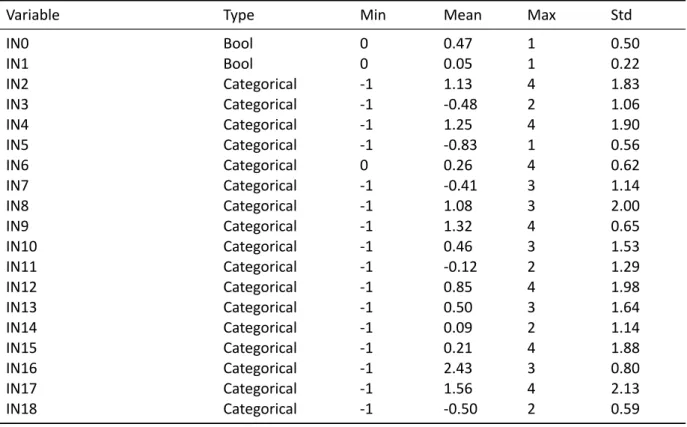
Data in Credit Scoring includes personal information about the individuals processed. To account for the sensitivity of the data, that is to protect the confidentiality and to concur with data protection reg-ulation, alterations are conducted. Hence, the variables are renamed to IN0 - IN18 and their meaning is only explained briefly and in a general sense. Additionally, the data set is weighted to incorporate more observations who turned out to be bad than in the real population. A benefit of the weighted data set is that because credit scoring mainly aims at the identification of bads in the population, it is important to include an adequate volume of bads to capture their structure in the model development process. The bads are represented by a performance measure, with 15 335 (≈27%) defaults on payment.

Brief explanation of the variables used

• IN0

Binary variable with information whether a customer is known to the client. • IN1

Binary variable with information whether shipping address and billing address match. • IN2

Elapsed time in days since the customer was registered by the system for the first time. • IN3

Validation of the billing address, i.e. whether the address exists and a customer is known to live at the stated address

• IN4 - IN5; IN10; IN11; IN13 - IN15; IN18

Information about the order history of a customer • IN6 - IN8

Information of the dunning history of a customer. • IN9

Discretized order value in relation to the clients’ average order value. • IN12

This variable is designed as means of fraud prevention. A fraudulent customer may employ a couple of orders with little order value to be known by the system as a good customer and subsequently employ expensive orders using insecure payment methods. Hence, the order value is compared to the average of past orders by the customer.

• IN16

Clock hour of order time. • IN17

In order to efficiently obtain the discriminant function the 13 continuous variables need to be discretized (Ong et al., 2005). The discretization is done using the Weight of Evidence (WoE) measure to assess the predictive power of each attribute. The WoE measures the difference between the distribution of goods and bads and therefore represents an attributes’ power in separating good and bad observations (Siddiqi, 2006). The WoE is frequently used in credit scoring to convert a continuous variable into a discrete variable and as such the used method at AFS.

The WoE is calculated as follows:

WoE=

lnDistribution Good_{Distribution Bad} ×100 (1)

A bin with a WoE around zero has the same probability of observing a default in payment as the sample average. Contrarily, if a bin has a WoE above or below zero, the probability of observing a default in payment is above or below sample average respectively. However, more important than the absolute WoE is the difference between bins. The variables predictive power relates to the difference in WoE between bins. Monotone bins offer a direction of effect over the bins. With monotone increasing WoE the probability of default is always higher in a greater bin and vice versa with monotone decreasing bins (Siddiqi, 2006). The interval boundaries of the bins are selected such that the bins are monotone increasing or decreasing, the differences in WoE over the bins are roughly equal, the bins are as evenly sized as possible and a minimal number of observations is maintained in each bin. Missing values are not submitted to the bin selection phase but treated as a separate bin exhibiting a value of -1. The reasoning for treating missing data this way is to account for its predictive value. Table 1 shows the discretization of continuous variables with the value ranges for the respective bins. Figure 9 shows the Table 1: Discretization of Continuous Variables

Variable -1 1 2 3 4

IN2 ∅ _{[−∞,90) [90,380) [380,600) [600,∞)}

IN9 ∅ _{[−∞,150) [150,300) [300,∞)}

IN17 ∅ _[−∞,25) [25,30) [30,40) [40,∞)

IN14 ∅ _{[−∞,18) [18,∞)}

IN15 ∅ _{(∞,7) [7,4) [4,2) [2,−∞)}

IN13 ∅ _[−∞,1) [1,4) [4,∞)

IN4 ∅ _{[−∞,1) [1,4) [4,10) [10,∞)}

IN5 ∅ _[−∞,∞)

IN10 ∅ _[−∞,5) [5,20) [20,∞)

IN11 ∅ _{(∞,6) [6,−∞)}

IN12 ∅ _{(∞,50) [50,25) [25,10) [10,−∞)}

IN16 ∅ _[−∞,9) [9,14) [14,∞)

The IV is calculated as follows:

IV=X

i(Distribution Goodsi−Distribution Badsi)×ln

Distribution Goods i Distribution Badsi

(2)

From the 12 discretized variables, 3 have an IV of less than 0.05, namely ’IN9’, ’IN16’ and ’IN5’. Nonethe-less, they are not removed from the data set, because while they seem insignificant by themselves, they might become more important in interaction with others. Furthermore, GP selects the important vari-ables automatically (Ong et al., 2005). The final dataset is shown in Table 2.

Table 2: Input Variables

Variable Type Min Mean Max Std

IN0 Bool 0 0.47 1 0.50

IN1 Bool 0 0.05 1 0.22

IN2 Categorical -1 1.13 4 1.83

IN3 Categorical -1 -0.48 2 1.06

IN4 Categorical -1 1.25 4 1.90

IN5 Categorical -1 -0.83 1 0.56

IN6 Categorical 0 0.26 4 0.62

IN7 Categorical -1 -0.41 3 1.14

IN8 Categorical -1 1.08 3 2.00

IN9 Categorical -1 1.32 4 0.65

IN10 Categorical -1 0.46 3 1.53

IN11 Categorical -1 -0.12 2 1.29

IN12 Categorical -1 0.85 4 1.98

IN13 Categorical -1 0.50 3 1.64

IN14 Categorical -1 0.09 2 1.14

IN15 Categorical -1 0.21 4 1.88

IN16 Categorical -1 2.43 3 0.80

IN17 Categorical -1 1.56 4 2.13

:R( ,1 ,QIRUPDWLRQ9DOXH &RXQW :R( ,1 ,QIRUPDWLRQ9DOXH &RXQW :R( ,1 ,QIRUPDWLRQ9DOXH &RXQW :R( ,1 ,QIRUPDWLRQ9DOXH &RXQW :R( ,1 ,QIRUPDWLRQ9DOXH &RXQW :R( ,1 ,QIRUPDWLRQ9DOXH &RXQW :R( ,1 ,QIRUPDWLRQ9DOXH &RXQW :R( ,1 ,QIRUPDWLRQ9DOXH &RXQW :R( ,1 ,QIRUPDWLRQ9DOXH &RXQW :R( ,1 ,QIRUPDWLRQ9DOXH &RXQW :R( ,1 ,QIRUPDWLRQ9DOXH &RXQW :R( ,1 ,QIRUPDWLRQ9DOXH &RXQW

4.2 Genetic Programming

Genetic Programming (GP) is an optimization method in the research field of Evolutionary Computa-tion, that adopts the Darwinian principles. Next to GP, the field includes a number of different methods among which are Genetic Algorithms, Evolution Strategies, and Evolutionary Programming (Eiben and Schoenauer, 2002; Eiben and Smith, 2015).

Genetic Programming (GP) is a domain independent evolutionary computation method that automat-ically finds a solution in a predefined search space. This is done by creating a population of computer programs that is stochastically transformed over time into a new population of computer programs by employing evolutionary mechanisms such as inheritance, selection, crossover and mutation, that are inspired by Darwin’s theory about evolution. GP computer programs are usually depicted in a tree rep-resentation, with variables and constants as leaves of the tree and arithmetic operations as internal nodes. In the GP setting, the former are called terminals and the latter functions. Together they form the primitive set. All computer programs that can be constructed by a primitive set define the search space of possible solutions (Koza, 1992). For illustration, figure 10 represents the syntax tree of the pro-gram(var1 +var2)∗2, withvar1,var2and2as terminals and+and∗as functions. In credit scoring,

x

+

var1 var2 2

Figure 10: Example Syntax Tree

these computer programs are discriminative functions that aim at assigning the associated probability of default to a customer. Hence, the problem is defined as a symbolic regression problem. Based on its output value, an appropriate threshold value can be chosen to classify customers into bads and goods. In this work, the function set consists of arithmetic operators, equality operators, relational operators and logical operators. Constants are included as terminals according to the values in the variable ranges from -1 to 4. Additionally, in order to allow for operations that decrease the impact of parameter values, decimal point constants between 0 and 1 are included as well. The GP parameter settings are shown in Table 3 and thoroughly explained below.

Table 3: GP Parameter Settings

Parameter Value

Population Size 300

Initialization Ramped Half-and-Half Fitness Function Area Under the ROC Curve

Function Set {+,−,×,÷,≤,≥,=,6=, if −then−else}

Terminal Set {Attributes,₁₀p |p∈N_∧p <10∪x∈Z_{∧ −1≤}x≤4}

Maximum Number of Generations 500

Selection Tournament

Crossover Rate 0.9

The process of GP is as follows. First, an initial population is created (Subsection 4.2.1). Next, GP enters the evolving process, starting with the evaluation of the population (Subsection 4.2.2). Based on the evaluation, functions are selected from the population (Subsection 4.2.3). Finally, the selected popula-tion is evolved using genetic operators (Subsecpopula-tion 4.2.4). The evolving process repeats until a satisfac-tory function is evolved or a maximum number of 500 generations have passed. The process of GP is depicted in figure 11 and thoroughly explain below.

INITIALIZE

POPULATION EVALUATE CONVERGENCE YES SOLUTION

SELECTION NO

GENETIC OPERATORS

4.2.1 4.2.2

4.2.3 4.2.4

Figure 11: GP Process

4.2.1 Initialization

4.2.2 Evaluation Criteria

A classification model maps observations to predicted classes. That is, a model predicts if an observation is good or bad. The GP model returns a continuous output to which different threshold, or cut-off points, can be applied in order to allocate the output to a class. Evaluating the prediction of an observation in respect to its true class provides four possible outcomes:

• True Positive - observations classified as bads whose true class membership is bads • False Positive - observations classified as bads whose true class membership is goods • True Negative - observations classified as goods whose true class membership is goods • False Negative - observations classified as goods whose true class membership is bads

Commonly, those outcomes are disposed in a confusion matrix (also called a contingency table), as depicted in figure 12. The outcomes with a ’true’ in their names, that is True Positive and True Negative’, represent correct classification and the outcomes with a ’false’ in their names, that is False Positive and False Negative’, represent incorrect classification. From the confusion matrix a number of metrics can be calculated. Some of those metrics are shown in equations 3 to 6 and explained below.

False Negative True

Positive

False Positive

True Negative Prediction Outcome

Bads Goods

Bads

Goods

T

ru

e

V

a

lu

e

Figure 12: Confusion Matrix

True Positive Rate (TPR)= True Positive

True Positive+False Negative (3)

False Positive Rate (FPR)= False Positive

False Positive+True Negative (4)

Precision= True Positive

True Positive+False Positive (5)

Accuracy (ACC)= True Positive+True Negative

The ROC curve is a two-dimensional graph that quantifies the performance of a classifier in reference to all thresholds (Yang et al., 2004). For this purpose, the relative frequency of every unique score value specified by the True Positive rate (TPR), i.e. the proportion of actual positives predicted as positive as depicted in equation 3, and the False Positive rate (FPR), i.e. the proportion of actual negatives pre-dicted as positive as depicted in equation 4, is plotted on the X and Y axis respectively (Baesens et al., 2003). Therefore, the ROC graph shows relative trade-offs between benefits and costs.

Figure 13 depicts an example representation for a ROC curve. The point in the lower left corner depicts a threshold that classifies all observations as goods. Such a classification induces no false positive error, but no true positives either. Contrarily, the point on the upper right corner corresponds to a threshold that classifies all observations as bads. Hence, both false positive and true positive are at their max-imum value. A perfect classifier incorporates a point in the upper left corner that classifies bads as bads and goods as goods. In general, a point with higher TPR and lower FPR compared to another is said to be better (Fawcett, 2003). In order to compare different models the ROC curve can be reduced

0.0 0.2 0.4 0.6 0.8 1.0

False Positive Rate 0.0

0.2 0.4 0.6 0.8 1.0

True Positive Rate

Receiver Operating Characteristic

Figure 13: Example ROC curve

to its single-scalar representation by calculating the AUC using the equation in 7. Because ROC-AUC takes the whole area under the ROC curve into account, it is possible for a classifier to be better than another in a specific region but have a worse ROC-AUC (Fawcett, 2003). The ROC-AUC represents the probability that a randomly chosen positive observation is ranked higher than a randomly chosen negative observation, which corresponds to the quantity of a Wilcoxon test (Hanley and McNeil, 1982; Baesens et al., 2003).

Area under the ROC curve (ROC-AUC)=

Z ∞

−∞

TPR(T)FPR′(T) dT (7) where T in (7) is a threshold parameter.

Since with advancing generations models grow in size until they reach a point from which it becomes increasingly difficult for humans to read and understand, measures to control model size have to be implemented. First, the models are being pruned once they reach a certain size. Second, the fitness is being expanded to a multi layered fitness by incorporating a secondary fitness on basis of model size. However, because ROC-AUC is the primary fitness function, only models with equal ROC-AUC are being compared on their size (Eggermont et al., 2004). In addition to keeping models small, size as fitness keeps variables out that have no effect on the models’ predictive power. Without size as fitness, models with attributes that have neither positive nor negative effect on the models’ predictive power have the same chance of survival as the models without. Contrarily, if size is implemented as fitness, models with attributes that have no predictive power have a lower chance of survival than models without. Therefore, size as fitness does not only keep models small but reduces the number of low performing attributes.

4.2.3 Selection

After initializing the population of solutions and assigning a fitness value to them, the evolutionary process of creating a new population of solutions can be started. In a first step solutions are being selected to be submitted to subsequent processing. The selected solutions represent the basis for the functions in the next generation. They are probabilistically selected from the population on the basis of their fitness, i.e. the higher the fitness of a function, the higher the probability that it gets selected. As a result, solutions with high fitness values have a higher chance of survival and propagation of their genetic material. The degree of preference to which a better solution is selected is called selection pressure. The selection pressure impacts the convergence rate, i.e. the rate of approaching an optimal solution. However, if the convergence rate becomes to high the search space is not explored thoroughly. In this case, the loss in diversity results in the premature convergence on a local optimum and prevents the evolutionary process of reaching the global optimum. On the other hand if the selection pressure is too low the time needed to converge to the global optimum increases which may lead to the stagnation of the evolutionary process.

Selection methods can be divided into proportionate-based and ordinal-based selection (Miller and Goldberg, 1996). Proportionate-based methods select solutions on the basis of their fitness, while in ordinal-based selection solutions are ranked according to their fitness and selected on the basis of their position in the ranking. The most well known selection algorithms are proportional selection, linear ranking selection and tournament selection and many more are presented in research.

Originally, selection was introduces by Holland (1975) with proportional selection. In this method, the probability with which a solutioniis selected is proportionate to its fitness value, i.e.

pi= fi PN

k=1fk

(8)

Deb, 1991; Blickle and Thiele, 1995a; Eiben and Smith, 2015). Grefenstette and Baker (1989) introduced linear ranking selection to overcome the drawbacks of proportional selection. In linear ranking selection the solutions are ranked by their fitness values, with the weakest solution ranked first and the strongest solution ranked last. Different ranks are distributed even for solutions with equal fitness. The selection probability is linearly assigned according to their rank, i.e.

pi =

1 N

2−η++ 2η+−2 i−1 N −1

;i∈ {1, ..., N} (9)

η+is the selection bias to adjust the selection pressure, with

1 ≤η+

≤2(Blickle and Thiele, 1995a). The selection pressure increases with increasingη+.

The most common selection method, called tournament selection is being used in this work. Although tournament selection is shown to be superior in regards to many other selection methods including the ones mentioned above, the reasons for the continuing popularity are found in its inherit features (Blickle and Thiele, 1995b). Tournament selection is very efficient for both parallel and non-parallel systems and it does not require the population of solutions to be sorted. Thus, it has a linear time com-plexity ofO(N)(Fang and Li, 2010).

Goldberg and Deb (1991) attributes the origins of tournament selection to ”unpublished work by Wet-zel” that was cited by Brindle (1981). In tournament selection, a tournament is being held between a number of functions in which their fitness values are compared. The function with the highest fitness value is declared winner and inserted into a mating pool. The functions in the mating pool incorporate a higher average fitness value than the entire population (Koza, 1992; Poli et al., 2008; Goldberg and Deb, 1991). However, because tournament selection selects the functions to compete randomly, every function in the population has a chance of being selected, which lowers the chance of getting stuck in a local optimum, which is known as premature convergence (Eiben and Schoenauer, 2002). In the process of comparing fitness values between functions, tournament selection only takes into account if a function is better than another but not by how much. This holds the degree to how much the better functions are preferred constant (Poli et al., 2008). This effect is called selection pressure (Miller and Goldberg, 1995). The advantage is that extremely powerful functions do not lead to loss in diversity and subsequently premature convergence in an suboptimal solution. However, the convergence rate is lower compared to methods with higher selection pressure and marginal advantages in performance are enough to be selected, which might exclude functions with helpful subtrees (Miller and Goldberg, 1995; Poli et al., 2008). Another way to influence the selection pressure is by altering the size of a tournament. While tournaments are regularly held with pairs of functions, the size may be increased. Decreasing the size to 1 does not make sense, because it results in uniformly random selection. In-creasing tournament size has an boosting effect on selection pressure because the probability that a high-fitness function is selected increases (Goldberg and Deb, 1991; Miller and Goldberg, 1995; Eiben and Smith, 2015). However, an increase of tournament size also increases the loss of genetic diversity. This work induces only low additional selection pressure by increasing the tournament size to include three functions.

4.2.4 Genetic Operators

functions with a higher discriminative power within the search space. The main genetic operators are called crossover and mutation.

The objective of crossover is to merge interesting but different information from two functions into a new function that combines these information. Hence, two discriminant functions from the population are selected and parts of their syntax tree is exchanged between them. Applied in this work is one-point crossover, in which a subtree from a selected function is replaced by a subtree from another selected function. The crossover point is randomly chosen, hence crossover is a stochastic operator (Eiben and Smith, 2015; Poli et al., 2008). While many other types of crossover are possible, DEAP only supports one-point crossover. Figure 14 depicts the genetic operators. Next to crossover, mutation is applied on

Randomly Generated Subtree

x

+

var1 var2 2

/

*

var1 2

-var3 5

+

var1 var2 /

-var3 5

-+

var1 var2 2

-2

-var1 _x

2 var2

-var1 _x

2 var2 Mutation Crossover

Figure 14: Genetic Operators

Koza (1992) argued that the use of mutation in GP is of no avail and only crossover should be used. How-ever, a number of studies showed that mutation does have utility and sometimes even outperformed crossover (White and Poulding, 2009; Angeline, 1997). While crossover and mutation can be used ex-clusively, they are not mutually exclusive and can be used in combination, which often times lead to better results (Luke and Spector, 1998). Hence, crossover is applied with 90% probability and mutation with 10% probability.

4.3 Applying Genetic Programming

Figure 15 shows the median fitness of the best functions in every generation over 5 runs during the evolutionary process on the training set as depicted in figure 11. The evolutionary process ran for 500 generations before being terminated. The fitness increases heavily for the first≈200 generations. For

the later≈300 generations, fitness only increases marginally. The performances of the best functions

of every run are validated on the validation set in order to verify their robustness.

*HQHUDWLRQ

)LWQHVV

0HGLDQ)LWQHVVRYHUDOO5XQV

Figure 15: Median Fitness over all Runs

Figure 16 depicts the model with the highest fitness value after termination of the evolutionary process. The model has a bushy shape and a size of 220 nodes with a maximal tree depth equal to the depth limit of 17. Bushy models are frequently observed using ramped half-and-half as initialization method (Poli et al., 2008). The two subtrees from the root are very different sized, with 193 and 27 nodes. Examining the tree shows that pruning can be employed at a number of nodes in order to reduce the size of the model. Pruning the model yields a size of 154 nodes and a maximal tree depth of 16 nodes. Most noticeable, the if-then-else nodes yield no utility but additional size, because every if-then-else node is connected to a boolean True/False decision terminal. Those nodes can be replaced by their subsequent node, i.e. if−then−else(F alse,IN12,IN16) ⇒IN16. Additionally, some subtrees are

Missing values are encoded as the value -1 that is not used in the model. Thus, the model does not specifically account for missing values.

Because GP automatically chooses important variables, one may conclude that the number of occur-rences gives information about the predictive power of a variable. From the 19 variables in the function set, six are not used in the model or used in combination with the if-then-else nodes on the unused side, which effectively removes them from the model. Those variables are IN1, which contains information whether shipping address and billing address match, as well as variables IN5, IN11, IN14, IN15 and IN18 that contain information about the order history of a customer. The remaining order history variables, IN10 and IN13, are incorporated into the model but only occur a single time in the model. Hence, order history provides little to nothing in additional discriminatory power.

Among the most often used variables are IN7 and IN6 with 13 and 9 occurrences. These variables, to-gether with IN8 which only occurs twice, contain information about the dunning history of a customer. A logical conclusion is that customers with prior payment difficulties are more likely to default than those without. Despite the low occurrence of IN8, dunning history provides a great deal of discriminatory power. With 10 occurrences, another heavily used variable is IN2 which contains information about the number of elapsed days since a known customer was registered by the system for the first time. This puts emphasis on continuous business connections between client and customers. Customer who have been customer for a long time are less likely to default on payment than first-timers. Finally, the fraud-prevention variable IN12 and IN16, which contains the order time, occur 5 times. The remaining variables are used between 1 and 3 times. Table 4 shows the variables with their respective occurrences in decreasing order.

Subsequently, the function with the highest fitness is passed on to be calibrated as depicted in figure 8. Table 4: Occurrences of Variables

Variable Number of Occurrence

IN7 13

IN2 10

IN6 9

IN12; IN16 5

IN3; IN4; IN17 3

IN0; IN8 2

IN9; IN10; IN13 1

+ x 0.5 -IN12 -x IN0 IN7 IN7 / -IN6 -/ IN2 IN4 -+ IN12 x -0.3 -IN2 x IN4 + x 0.7 0.3 IN7 IN7 x 0.5 IN2 IN7 -IN2 IN6 x IN6 -IN13 IN7 / if

False IN9 IN16

/ / + IN16 / if True / if True / IN7 -/ if

True IN17 0.5

-0.5 IN3 IN6 1.0 -/ if

True IN17 IN15

-0.5 IN10

IN6 if

True IN2 IN15

/ 2.0 0.4 + -IN2 -IN2 -IN2 x 0.7 0.3 -if

False IN12 IN8

if

False IN6 IN16

IN6

-x

0.5 IN7

if

True 0.5 0.5

0.7 / if True / if True / x 0.3 IN7 -IN3 0.7 IN16 -IN3 0.7 IN10 / IN0 / 2.0 0.4 x 0.3 0.4 / / IN9 / if

False IN12 IN16

/ / 2.0 + IN16 / if True if True / IN8 -/ if

True IN17 IN16

4.4 Calibration

The output from GP can be used to rank the order from least to most probable default. However, these scores do not represent an accurate estimate of the probability. Calibrating the outputs allows for the score to be interpreted as a probability. Probabilities are needed for two reasons. First, the GP outputs are supposed to be used as an on-top addition or deduction to the credit agency score which represents a probability. Second, the outputs are eventually not going to be used solely by itself but in combination with misclassification costs (Zadrozny and Elkan, 2001).

In order to calibrate the GP outputs a non-parametric type of regression called Isotonic Regression (IR) is used. Among the models’ benefits is the lack of assumption about the form of the target function. However, IR assumes that the classifier ranks the observations properly. The IR problem is defined by finding a function that minimizes the mean-squared error (Zadrozny and Elkan, 2002; Niculescu-Mizil and Caruana, 2005):

minX

i(yi−f(xi)) 2

(10) IR uses pair-adjacent violators (PAV) to find the best fitting stepwise-constant isotonic function, which works as follows. For every observationxi, the value of the function to be learnedf(xi)must be bigger or equal tof(xi−1). Otherwise the resulting function f is not isotonic and the observationsxiandxi−1 are called pair-adjacent violators, hence the name of the algorithm. In order to restore the isotonic assumption, bothf(xi)andf(xi−1)are replaced by their average. This process is repeated with all observations until no pair-adjacent violators remain (Ayer et al., 1955).

In the setting of Credit Scoring, PAV works as follows. First, the observations are ordered according to their score values. Then, thef(xi)is set to 0 ifx1belongs to the goods, andf(xi)is set to 1 ifx1belongs to the bads, respectively. If the score ranks the examples perfectly, all goods come before bads and the values offare unchanged. As a result, the new probability estimate is 0 for all goods and 1 for all bads. Contrarily, in a random scoring system that does not incorporate any information about the ordering, the probability estimate will be a constant function with the bads rate as value. PAV provides a set of intervals with a corresponding set of estimatesf(i)for every interval i. In order to use the results on new data, a probability estimate is mapped to an observation according to its corresponding interval, for which the score value is between the lower and upper boundary (Zadrozny and Elkan, 2001). In order apply IR on the uncalibrated GP output data set, the validation set is used to train the IR classifier using 10-fold cross-validation. The classifier is subsequently employed on the test set as depicted in figure 8. Below, the calibration plots in figure 17 illustrate the process of calibration on the training set in the Isotonic Regression Plot, how well the resulting set of isotonic values is calibrated on the test set in a reliability curve and the respective distribution of score values in a histogram.