1
Productivity, Wages, and the Returns to Firm-Provided
Training: Fair Shared Capitalism?
Abstract
In this study, we develop an alternative modelling that examines a) the determinants of firm productivity and wages and b) the internal rate of return (IRR) to firm training for both firms and workers. Using a six-year linked employer-employee dataset, our estimates indicate that an additional hour of training per worker results in an increase of 0.12% in productivity and 0.04% in wages, or an increase of 0.16% and 0.08%, respectively, if one uses firm training as a stock variable. We then find that 82% of the gains in productivity are captured by firms and 18% by workers. Given the training costs, we finally obtain an IRR of 13% for firms and 33% for workers at sample means. Firms are heterogeneous, and we do find that dispersion in the rates of return across firms is high.
JEL classification J24, J31, I2 Keywords
Firm-Provided Training, Internal Rate of Return, Human Capital, Productivity, Wages
Word count
2
1. Introduction
Despite a lack of reliable international data, it is fairly safe to say that the investments that firms make in human capital through formal training can be as high as 3% of total labour costs (Bassanini et al. 2007). Since the costs of most of these training programmes are born by firms, either directly by paying all direct costs (e.g. fees paid to training institutions), or indirectly through a loss of working time, firms are expected to capitalise on their investment in training through higher productivity. However, firm-sponsored training, whether general or firm-specific, would not be worthwhile if workers were allowed to use up all of the productivity gains by receiving higher wages. The need for training investments to be worthwhile seems to be self-evident, as otherwise they would not even be considered by companies, but it remains to be seen the extent to which the productivity gains associated with workplace training are shared by both the firms concerned and their workers.
The novelty of our approach is that the gains enjoyed by firms are computed as net gains – i.e. net of the training costs on the one hand, and net of all the gains accruing to workers through higher wages on the other. The wage gains are obtained from a wage equation and the training costs estimated from a training cost function. Both are fitted to firm-level data. We model, therefore, the impact of an additional hour of training on both productivity and wages in a unified framework. Then, in order to compute the internal rate of return for workers and firms, we take into account that training participants sacrifice a fraction of their leisure time, while at the same time firms support all the direct training costs, as well as the foregone output associated with having training sessions during normal working hours. The key aspect in our modelling is that it allows us to derive an explicit formula for the internal rate of return for firms and workers. As far as we know this is the first time that such an approach has been used. Confirming our priors, in the case of the firms’ returns to training the model predicts that the rate of return is associated positively with the elasticity of output with respect to training hours and negatively with the elasticity of training costs with respect to training, the foregone output, the wage gains, and the rate of depreciation. For workers, the internal rate of return depends directly on the elasticity of wages with respect to training and inversely on the size of the workers’ opportunity costs.
Empirically, we observe that most firms do indeed benefit from training in net terms. In fact, 86% of all training firms have a positive internal rate of return, while on aggregate we estimate that the internal rate of return for firms is 13%. Since the training costs for workers are small, the corresponding net gains evaluated at sample means are more pronounced, at 33%. We also estimate that workers capture approximately 20% of the estimated productivity
3 gains. Overall, our results confirm that training does matter, as has been shown in many previous studies (e.g. Bartel, 2000, Pischke, 2005, Frazis and Lowenstein, 2005, Leuven, 2005, Ballot, Fakhfakh, and Taymaz, 2006, Dearden, Reed, and Van Reenen, 2006, and Bassanini et al, 2007).
Our main contribution is to derive a unique and distinct analytical framework for the determinants of the internal rate of return to firm-sponsored training. A recent study by Almeida and Carneiro (2009), for example, examines the internal rate of return to the investment that firms make in training very extensively but derives no explicit internal rate of return. The corresponding returns for firms are not net of the wage gains obtained by workers, nor is the return rate for workers modelled. However, a great deal of effort goes into estimating production and cost functions. Our modelling of the wage equation is also inspired by Dearden, Reed, and Van Reenen (2006), while the analysis of the workers’ and firms’ shares of the productivity gains is based on Ballot, Fakhfakh, and Taymaz (2006). Finally, unlike Dearden, Reed, and Van Reenen, our analysis is carried out at the firm, rather than sector level, while the work carried out by Ballot, Fakhfakh, and Taymaz put forward a totally different rationale for the firm-level wage equation. On the whole, we believe that our integrated modelling is appealing as it shows the key aspects at stake in a unified framework. Our treatment of the stock of training variable also includes some improvements on those to be found in extant literature.
This paper is organized as follows: In the next section, we present the modelling strategy used to evaluate the relation between productivity/wages and firm-provided training, which is based on an augmented Cobb-Douglas production function. Then, we investigate the relationship between training costs and training intensity and present the framework required to control the unobserved heterogeneity of firms, as well as a full derivation of the internal rate of return to training for workers and their firms. Section 3 describes our dataset and Section 4 presents the results. The main conclusions are drawn in Section 5.
2. Modelling
2.1 The impact of training on productivity and wages
Consider a Cobb-Douglas production function given by:
, (1.1)
Zjt ujt
jt jt jt jt
Y AH K Tr e
4 stock of capital; Tr is the number of hours of firm-sponsored training and Z denotes the vector of time-variant and time-invariant firm characteristics, including information regarding workforce composition. u is the error term and subscripts j and t are firm and period (year) identifiers, respectively.
By dividing equation (1.1) by H, we obtain the hourly productivity of labour,yjt, given by: jt 1 , (1.2) jt Z u jt jt jt jt y AH k tr e
where k and tr denote capital and hours of training per hour of work, respectively. Taking logs from equation (1.2), we have:1
log yjt log A( 1) log Hjtlog kjtlog trjtZjtujt. (1.3) Following the literature (e.g. Hellerstein, Newmark and Troske, 1999, Dearden, Reed and Reenen, 2006, and Ballot, Fakhfakh and Taymaz, 2006), we use a common set of regressors in the log hourly wage and productivity equations. Thus, using equation (1.3), we have:2
log wjt log Aw log Hjtwlog kjtlog trjt wZjtjt. (1.4) As with parameter in model (1.3), in model (1.4) is expected to be positive, that is, we anticipate that training will have a positive impact on the hourly wage. Whether is higher or lower than is another matter to which we shall turn to below.
2.2 Controlling for unobserved firm heterogeneity
We deal with unobserved firm heterogeneity by assuming that the error term in jt model (1.4) is given by jt j ejt, where ejt is i.i.d. and is the unobserved firm fixed-j effect. Then, using matrix notation, (1.4) becomes:
logW XG e, (2.1) where G denotes a JTJ matrix of dummies representing the set of J firms in the sample, T is the length of the panel, and
5
11 11 11 11
12 12 12 12
log 1 log log log
1 log log log
* . ... 1 log log l og w w JT JT JT JT w A H k tr Z H k tr Z X H k tr Z
Multiplying (2.1) by MG, with MG I PG and PG G G G( T ) 1GT
, we have:
log . (2.2)
G G G G
M W M XM G M e
By definitionM GG 0, which leads us to:
^ 1 log . (2.3) T T G G X M X X M W Then using equation (2.1), we have:
^ 1 ^ log . (2.4) T T G G G W X which can be rewritten as:
^ 1 ^ ^ ^ ^ ^
log log log log log . (2.4')
T T
j G G G wjt Aw Hjt w kjt trjt wZjt
Equation (2.4) – or (2.4’) – indicates that we measure the unobserved firm effect by using the difference between the observed average wage of the firm and the expected average wage, given X, where X denotes the full set of firm- and worker-level characteristics.
Finally, adding ˆj to models (1.3) and (1.4), we obtain:
^
log yjt log A( 1) log Hjtlog kjtlog trjtZjt jjt, (2.5) and
^
log wjt j log Aw log Hjtwlog kjtlog trjtwZjtejt. (2.6)
6 our treatment ultimately controls for a possible correlation between the unobserved ability of workers and their participation in training. This is, of course, a non-trivial notion.
Finally, since the effects of training are expected to last for more than one period, we derive an alternative stock measure, which is given in the appendix. The estimated stock variable then allows us to examine the effect of lagged training on the current productivity level. The results in Section 4 below use the two training variables for comparison purposes.
2.3 Training costs
Following Frazis and Loewenstein (2005), we use the Box-Cox transformation to investigate the appropriate functional form for the direct costs of training. Accordingly, we specify the training cost as a function of
Tr1 /
– where, again, Tr denotes the hours of training – and obtained ˆ 0.09, which is estimated using non-linear least squares. Given this evidence, the following log-log training cost function was assumed:0
logCTrjt log logTrjtcZ'jtjt, (3.1)
where CTrjt denotes the direct training costs of firm j in period t (net of public subsidies). Z’ denotes observed firm characteristics, including capital and hours of work. In this equation, gives the elasticity of direct training costs with respect to hours of training.
To calculate the foregone value of production – i.e. the indirect costs resulting from the fact that training often occurs during normal working hours – we return to equation (1.1) (subscripts j and t being omitted) and specify that:
[ ( )] Z u. (3.2)
Y A H Tr K Tr e
In this framework, the (negative) indirect effect of training on value added is obtained via [H Tr( )], so that we have: , (3.3) Y dH Y dH H dTr H dTr
7
where Y H
H Y
indicates the elasticity of output with respect to hours. Based on (3.3), the
derivative dH
dTr gives the relationship between the hours of work and hours of training, which is assumed to be negative as an increase in training hours produces a decrease in the number of hours spent on production. However, training is not always carried out during normal working hours, in which case we have the effect of training on hours given by
( ),
R
H Tr
Tr
where R denotes the number of hours subtracted from production due to training, with RTr. Thus, making dH H R
dTr Tr Tr
we have, in absolute value:
. (3.4) Y dH Y R R y H dTr H Tr H tr
2.4 The internal rate of return to training for firms
We model firm-sponsored training in a similar way to an investment in physical equipment. We further assume that training takes place in year t, while the productivity gains are felt in the post-training year t+1 up to period t+n. The training costs in turn are assumed to be fully paid in year t. Under this set of assumptions, the internal rate of return, r, is such that we have:3 1 , (4.1) (1 ) n t i t i i NMgB MgC r
where NMgB is the net marginal benefit of an additional hour of training and MgC is the corresponding marginal training cost. We emphasize that the internal rate of return in this case is net of any possible wage gain to workers. Thus, in contrast to Almeida and Carneiro (2009), in our case the rate of return for employers depends explicitly on the effects of training on productivity and wages, as well as on the training costs. In other words, our parameter of interest is the net benefit accruing to firms, while Almeida and Carneiro are only concerned with the productivity gains associated with an additional hour of training.
8 1 1 1 1 1 . (4.2) (1 ) (1 ) (1 ) n n n t i t i t i i i i i i t i t NMgB Y W r r Tr r Tr
where W is the annual wage bill.
Then, using the production function (1.1) and replacing Trt by the stock variable
t
M (see equation (A.2) in the appendix), we have:
2
1 2 1 + 1 +...+ 1 l Zt t , (4.3) t t t t t t t l Y AH K Tr Tr Tr Tr e where is the firm-specific depreciation rate. (Expression (A.5) in the appendix shows how the stock of training is calculated in practice.)4
Now, differentiating (4.3) with respect to Trt i we have:
(1 )i (1 )i , (4.4) t t t t i t t Y Y y Tr M m where t t t M m H .
Using equation (4.4) we can assume that t i (1 )i t
t t
Y y
Tr m
. Then, given that is
the elasticity of the hourly wage with respect to tr (by (2.6)), the marginal effect of training on wages can be given by t i (1 )i t
t t W w Tr m .
Thus, using (4.2), we have:
1 (1 ) (1 ) (1 ) (1 ) ... ... , (4.5) (1 ) (1 ) (1 ) (1 ) (1 ) n n n t i t t t t i n n i t t t t NMgB y y w w r r m r m r m r m
which is equivalent to:
1 (1 ) (1 ) ... . (4.6) (1 ) (1 ) (1 ) n n t i t t i n i t t NMgB y w r m m r r
Now, (1 ) ... (1 ) (1 ) (1 ) n n r r is a geometric series with n terms, and a common ratio
of 1 1 r
, and an initial value given by 1 1 r , yielding:
9 1 1 1 1 1 1 = 1 . (4.7) 1 1 1 1 1 n n r r r r r
Assuming n , we then have:
1 1 1 1 . (4.8) 1 r r r
Finally, we substitute (4.8) into (4.6) to obtain the present discount value of the net marginal benefit for firms:
1 1 . (4.9) (1 ) n t i t t i i t t NMgB y w r m m r
At this point we recall that the training costs contains two components, i.e. the direct cost and the foregone output. Firstly, the marginal direct cost of training can be computed using (3.1) to obtain: , (4.10) Tr Tr t t t t C C Tr Tr
while the marginal indirect cost is given by (3.4). Thus, combining (4.1) and (4.9), we have:
1 , (4.11) Tr t t t t t t t t t t t t y w C y R y m m r Y tr H tr
which is equivalent to:
1
, (4.12) t t y y t t t m w c s r tr with t y t t w w y , t Tr y t t C c Y , and t t t R s H .Further manipulation of (4.12) then gives us a general formula for the internal rate of return:
1 - . (4.13) t t y y t t t w r m c s tr 10 the elasticity of the value added with respect to training hours and, inversely, on a) the direct costs of training, b) the foregone output, c) the wage increases, and d) the depreciation rate.
2.5 The internal rate of return for workers
We assume that the direct costs of training are paid by employers. We also rule out the possibility of any nominal wage reduction during the training period. Given that we leave apprentices out of the estimation sample and that there is little evidence that workers pay indirectly for the training costs through lower wages (e.g. Bassanini, et al. 2007, p. 200), we do not find this set of simplifying assumptions too restrictive. However, if workers are trained outside normal working hours, that implies an indirect cost to those workers. We proxy this cost by using information regarding the overtime-pay premium observed in the data. We note that this information is not available in Balanço Social: it was obtained from Quadros de Pessoal instead (see section 3 below).5
The indirect cost to workers of training is therefore calculated as follows: firstly, we specify the overtime wage bill as a function of hours of work to obtain the corresponding elasticity, , given by wo , (5.1) o o o t t w t t W W H H where o t
W denotes the overtime wage bill.
Then, given that only a fraction ( t t) t
Tr R Tr
of total training hours occurs outside
normal working hours, the workers’ marginal indirect training costs are given by:
( ) , (5.2) o o o t t t t w w t t t t W Tr R w v H Tr tr with ( t t) t t Tr R v H and o o t t t W w H
. (vt is rather small in our sample, at 0.2%, on average.)
To compute the internal rate of return for workers, we next use the second term in the right-hand-side of equation (4.5) to obtain:
11 1 (1 ) (1 ) ... , (5.3) (1 ) (1 ) (1 ) L n n t i t i n i L t L L MgB w r m r r
where rL is the internal rate of return to training for workers.
Finally, we equate the marginal benefit of training in (5.3) to the indirect cost of training in (5.2) to yield:
1
- . (5.4) t o t L o t w t t w w r m v tr We now have, therefore, an explicit formula for the internal rate of return for workers (rL) that depends directly on the elasticity of the hourly wage with respect to training and inversely on both the depreciation rate and the indirect training cost. As expected, the latter indicates that the higher the percentage of training hours that occurs within standard working hours, the higher is the return to training enjoyed by workers.
3. The Data
Our main source of raw data comes from Balanço Social. This dataset has been collated by Gabinete de Estudos e Planeamento (GEP) of the Portuguese Ministry of Labour, and covers all firms having at least 100 employees in the business sector of the Portuguese economy. In particular, we follow all training firms for a period of six consecutive years, from 1995 to 2000 (annual data), where a training firm is defined as one that offered at least some type of training in every single year of the period under study. In the raw sample, some 50% of firms did not provide any training in at least one year of the 1995-2000 interval. These firms were excluded from the estimation sample and as a result we were left with a total of 1,030 ‘training’ firms, a subset representing approximately 30% of the total Portuguese business sector workforce.
Balanço Social provides us information regarding a number of relevant firm-level variables useful to our study such as: value added, capital depreciation, labour costs, the wage bill, the number of employees, hours of work, location, industry, and legal form. The data
12 base also provides information regarding the levels of schooling, tenure, and skills of the workforce. The information regarding the overtime premium was obtained from Quadros de Pessoal, a linked employer-employee dataset also collated by GEP.
A unique feature of Balanço Social is that it contains detailed information on formal training offered by firms, including the number of participants (by occupation) and the number of training hours by type (on- and off-the-job training).6 Direct and indirect costs of training are also provided by Balanço Social, with the latter being proxyied by R/H times the wage bill.
As shown in Table 1, which summarizes the training statistics, the proportion of total training hours (see column (3), first row) is approximately 1% of total hours of work, with most (i.e. 77%) of the training hours taking place during standard working time. On average, each worker spends approximately 16 hours per year in training. As one might expect, the dispersion across firms in the sample is very high, with more than fifty percent offering less than 8 hours of training per employee and year. Total training costs amount to 0.70% of total value added and the indirect costs, given by R/H times the wage bill, amount to 0.28%.7
(Table 1 near here)
Table 2 presents the mean and standard deviation of an extended set of firm-level variables grouped into two categories: firms with training hours above and below the median, respectively. Clearly, firms offering more intensive training have both a higher level of productivity and higher wages. They are also larger in terms of the number of employees and capital intensity, and show a higher level of schooling and skill content as well. Tenure is slightly higher in firms with an intensity of training that is above the median.
13
4. Results and interpretation
4.1 The impact of training on productivity and wages
The results obtained from model (2.5) are shown in Table 3, column (1). The R2 coefficient indicates that the model explains more than 75% of the variation in firm productivity. The parameter ( 1) is negative and statistically significant (at 0.1 level), pointing to the presence of a decreasing returns to scale technology. In turn, the elasticity of the (log) value added with respect to hours is equal to 0.69.8
(Table 3 near here)
The impact of training on value added per hour is given by the training variable coefficient. Thus, if firms double their number of training hours – i.e. increase them from 1% to 2% or 16 additional hours of training per worker (per year) – then productivity will increase by 1.8%. Alternatively, 10 hours of additional training per worker will increase productivity by 1.2%, an effect that is comparable to the results reported by Almeida and Carneiro (2009), who claim that 10 additional hours of training per worker result a 0.6 to 1.3% increase in productivity.9
Column (2) of Table 3 gives the results from model (2.6), where it is apparent that the higher the ratio of training hours to total hours, the higher are the (average) wages paid by the firm. This result suggests that workers do benefit from the gains achieved through firm-provided training. Not surprisingly, the coefficient of the training variable in column (2) is smaller than the corresponding coefficient in column (1).
Columns (3) and (4) of Table 3 replicate columns (1) and (2), but now use the estimated stock of training hours rather than the corresponding annual flow.10 As can been seen, using the stock variable produces an increase in the impact of training on productivity and wages. Note that by comparing columns (1) and (3) and (2) and (4), it follows that the training coefficients in the productivity equations are at least twice as big as the corresponding coefficients in the wage equations. These estimates compare well with those of Dearden, Reed and Reenen (2006), who found that the impact of training on productivity is twice as evident as its impact on wages.
14 In this context, it is also worthwhile obtaining a quick measure of the percentage of the productivity gains enjoyed by both workers and firms. Formally, since (i) the marginal gain in output associated with an additional hour of training is given by dY Y
dTr Tr and (ii) the marginal gain in wages is given by dW W
dTr Tr , it follows that the shares of the workers and
firms are given by W Tr Y Tr (or y w ) and
y
w , respectively.Using these formulae, and values of y
w = 0.37, = 0.025, and =0.012, the workers’ share is 18%, while the firms’ share is 82%. The workers’ share is therefore lower than that obtained by Ballot, Fakhfakh and Taymaz (2006) for Sweden and France, at 0.35 and 0.30, respectively.
Interestingly, the proportion of gains captured by workers from firm-supplied training is substantially smaller than, for example, the case of the investment in schooling, which is 27%. This result is not surprising given the general content (or portability) of the investment in formal education.
Next, we briefly report on the results obtained by applying models (2.5) and (2.6) to the subsamples of low- and high-training firms, which are defined as firms with training hours below and above the median, respectively. It seems that training has a greater impact on the productivity of firms with less intensive training, while the impact on wages is higher for firms that offer a more intensive training programme. However, the difference across the two groups of firms is smaller (in absolute value) in the latter case. In other words, training seems to improve the relative productivity of firms that engage in low levels of training and to slightly increase the relative wages of firms that offer more intensive training.
We finally test for the existence of training spillovers between workers in a given firm by investigating the extent to which low-skilled workers benefit from the training intensity of
15 highly-skilled workers.11 To this end, we specify a model in which the dependent variable is
the average hourly wage of unskilled workers. The right-hand-side variables are the same as in model (2.6) but with two training variables: the training intensity of low- and highly-skilled workers, respectively. We found that the wage of low-skilled workers depend directly on their training intensity, as well as on the training intensity of the highly-skilled group. There seems to be therefore confirmation of the results obtained by De Grip and Sauermann (2012), pointing to the existence of externalities across co-workers. This evidence also underscores the importance of firm-level information as the effect of training will tend to be underestimated in worker-level data.
4.2 The training cost function
Table 4 shows the results from model (3.1). The coefficient of the training variable indicates that if, for example, firms duplicate the intensity of training, the direct training costs will increase by 66%, showing a relatively inelastic relationship between costs and training hours. Capital intensity, firm size, the proportion of skilled workers and their level of schooling also have a statistically significant impact on direct costs.
(Table 4 near here)
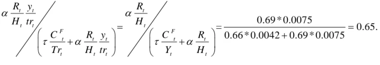
As mentioned above, indirect costs of training are based on the estimated loss of output. Thus, given that the direct and indirect marginal training costs are given by (4.10) and (3.4), respectively, our estimate, at sample means, of the percentage of the indirect marginal costs in total marginal training costs is given by:
0.69 * 0.0075 = 0.65. 0.66 * 0.0042 0.69 * 0.0075 t t t t t t F F t t t t t t t t t t R y R H tr H C R y C R Tr H tr Y H
16 That is, the forgone output represents 65% of total training costs, which is virtually the same percentage as the one derived from the raw data (see Section 3, footnote 7). Clearly, one cannot ignore the existence of the indirect costs of training.
4.3 Estimates for the Internal Rate of Return
Table 5, column (1), presents the summary statistics relating to the estimated internal rate of return for firms, r, obtained by using equation (4.13). The median of r is 30%, while the proportion of firms with a negative internal rate is 14%. The level of dispersion is also very high, an aspect that is associated with the high dispersion observed as companies invest in training as shown in Table 1.
(Table 5 near here)
We can also derive an aggregate internal rate of return at sample means. In this case, equation (4.13) yields:
1 0.025 0.012 * 0.37 * 0.81 - 0.19 0.125. 0.66 * 0.0042 0.69 * 0.0075 *6.5 t t y y t t t w r m c s tr Finally, in column (2) of Table 5, we give the summary statistics for the internal rate of return for workers, rL. The reported values are obtained by applying model (5.4) to a sample of firms in which the ratiovt, given by ( t t)
t
Tr R H
, is greater than 0.02%. Since a) workers do not bear any direct training costs, b) the estimated workers’ indirect costs of training are small, and c) workers were able to capture approximately 20% of the productivity gains, it is not surprising that the average rate of return for workers is very positive, at 62.5%. At sample means the internal rate of return is substantially lower, at 33%, which is of course much more palatable. Interestingly enough, we found no statistically significant correlation between worker and firm internal rates of return.
17
5. Conclusions
In this paper we derive firm-level productivity and wage models as a function of workplace training. The results obtained from our model specifications indicate that an investment in training has a positive and statistically significant impact both on productivity and wages. In particular, it is estimated that one additional hour of training per worker results in a 0.12% increase in productivity and a 0.04% increase in wages. These two effects become stronger if the selected training variable used is the stock of training rather than the flow. Furthermore, our estimates indicate that 80% of the gains in productivity are captured by firms and 20% by workers.
We have also derived a general model for the internal rate of return to training that, for the first time to our knowledge, addresses a) the effects of training on productivity and wages, b) the corresponding costs (both direct and indirect), and c) unobserved firm heterogeneity, all in a context in which a wide set of firm and worker-average characteristics are observed, including detailed information regarding training costs. Considering the subset of training firms, the internal rate of return for firms, at sample means, is 12.5%.
Training is good for workers too. In fact, the internal rate of return for workers at sample means is 33%, which, as expected, is higher than the rate of return for firms, as training costs are mostly born by firms. All in all, the estimated gains for both workers and firms are far from trivial, a finding that should encourage policy makers to treat firm training as a genuinely worthwhile investment.
18
Appendix
Let us consider the following expression:
1 , 1
, 1, (A.1)jt jt j t j t
M Tr M
where the stock of training in firm j at the end of period t (Mjt) is given by the amount of training offered in t (Trjt) plus the stock of training at the end of previous period (Mj t,1), adjusted by the firm-specific depreciation rate (j t,1). In our implementation, j t,1 depends on the observed job separation rate of firm j in period t-1, which is defined as the ratio of the number of separations observed in year t-1 to the number of employees in the beginning of the same year. We assume therefore that worker separation generates a loss in firm-specific human capital.
Using (A.1), we easily obtain:
2
, , 1 , 1 , 1+ 1 , 2 , 2+...+ 1 , , , (A.2)
l
j t j t j t j t j t j t j t l j t l
M Tr Tr Tr Tr
where l denotes the number of years of cumulative training. Parameter l is proxied by using the age of each firm, values of which are available in our dataset.
Furthermore, in our dataset, we have longitudinal information regarding the percentage of training hours in the total number of hours worked for the period 1995-2000 and regarding the corresponding separation rates for all firms in the sample. Additionally, assuming that the training flow before 1995 can be proxied by the 1995-2000 average, we then have, for t=1999 (or t = 99 to shorten the notation):
4 ,99 ,99 ,98 ,98 ,95 ,95 5 5 1 +...+ 1 + + 1 1 ... 1 , (A.3) j j j j j j l j j j j j j M Tr Tr Tr Tr Tr Tr where 1 1 T j jt t Tr Tr T
, 1 1 T j jt t T
, and T=6.19
4
5
5 ,99 ,99 1 ,98 ,98+...+ 1 ,95 ,95+ 1 1 1 ... 1 ,(A.4) l j j j j j j j j j j M Tr Tr Tr Tr which, by considering the geometric series with common ratio
1j
and initial value equal to 1, is equivalent to:
5 5 4 ,99 ,99 ,98 ,98 ,95 ,95 1 1 1 +...+ 1 + 1 . (A.5) 1 1 l j j j j j j j j j j M Tr Tr Tr Tr 20
ENDNOTES
1 Model (1.3) is similar to that described by Ballot, Fakhfakh and Taymaz (2006), equation
(2), except that we have used hours of work rather than the number of employees as the labour input. In our case, a standard test carried out on the statistical significance of the ( 1) term will indicate whether there are economies of scale in the production function.
2 A similar specification can be derived using a standard data generation process for worker
(log) earnings. Thus, if worker earnings are a function of both individual and firm characteristics, it then follows that a firm’s average wage will depend on worker average and firm-level characteristics too. We note that the rationale presented in Ballot, Fakhfakh and Taymaz (2006), for example, has a different micro foundation, being the equilibrium wage rate based on a Nash bargaining solution to the bargaining problem. The implications are nevertheless the same: both the wage rate and the labour productivity are ultimately determined by a common set of explanatory variables.
3 We omit the subscript j to simplify the notation. 4 We assume
jt j
, with given by the time average of the depreciation rate over the j sample period, to obtain a more parsimonious expression for the internal rate of return. Our results are not affected by this assumption.
5 In Quadros de Pessoal, and for the selected sample of firms, the observed average overtime
premium is 1.86 times higher than the standard hourly wage rate.
6 Our modelling does not separate on- and off-the-job components: for two main reasons: it
would considerably complicate the model derivations and, empirically, it would adversely affect the results due to the lack of information available from a sufficiently large number of firms.
7 Given that the wage bill is approximately 37% of the value added created by firms, the
forgone output due to training occurring within normal working time is 0.76% (= 0.28%/0.37). The actual share of indirect costs is therefore 64% (= 0.76/(0.76+0.42)), not 40% (= 0.28/0.70).
8 Using the results in the first column of Table 3, we have
1 0.033 1 0.258 0.018 0.033,
21
9 We do not find any statistically significant correlation between the change in sector-level
productivity and the firm-level training flow variable. This result indicates that the endogeneity of training is not obvious in the data.
10 The average proportion of the stock of training in total hours is 4.8%, which is six times
higher than the ratio of the training hours flow to total hours. The computation of the stock variable is strongly robust to changes in the depreciation rate. We tested several alternatives, including the case in which the depreciation rate is time-invariant and constant across firms, and found that the correlation across the different measures of the stock of training is always above 0.90.
11 Training participation figures are not available on an individual (worker) basis from
Balanço Social. Instead, the information regarding training is given according to skill groups, and that information allows us to find the percentage of a specific skill group that has actually participated in training sessions in a given year, as well as the corresponding number of hours spent on training. In turn, the average hourly wage by skill group is obtained using Quadros de Pessoal.
22
REFERENCES
Almeida, R. and Carneiro, P. (2009). The Return to Firm Investment in Human Capital. Labour Economics, 16(1): 97-106.
Ballot, G., Fakhfakh, F. and Taymaz, E. (2006). Who Benefits from Training and R&D, the Firm or the Workers? British Journal of Industrial Relations, 44(3): 473-495.
Bartel, A. (2000). Measuring the Employer’s Return on Investments in Training: Evidence from the Literature. Industrial Relations, 39(3): 502-524.
Bassanini, A., Booth, A., Brunello, G., Paola, M., and Leuven, E. (2007). Workplace Training in Europe. In G. Brunello, P. Garibaldi, and E. Wasmer (eds.), Education and Training in Europe, Oxford University Press.
De Grip, A., and Sauermann, J. (2012). The Effects of Training on Own and Co-Worker Productivity: Evidence from a Field Experiment. The Economic Journal, 122: 376-399.
Dearden, L., Reed, H. and Reenen, J. (2006). The Impact of Training on Productivity and Wages: Evidence from British Panel Data. Oxford Bulletin of Economics and Statistics, 68(4): 397-421.
Frazis, H. and Lowenstein, M. (2005). Reexamining the Returns to Training: Functional Form, Magnitude, and Interpretation. Journal of Human Resources, 40 (2): 453-76.
Hellerstein, J., Neumark, D. and Troske, K. (1999). Wages, Productivity, and Worker Characteristics: Evidence from Plant Level Production Functions and Wage Equations. Journal of Labour Economics, 17(3): 409-446.
Leuven, E. (2005). The Economics of Private Sector Training: A survey of the literature. Journal of Economic Surveys, 19(1):91-111.
23 TABLE 1
Firm-provided training, summary statistics
Variable On-the-job training (1) Off-the-job training (2) Training (On- and off-the-job)
(3)
Training hours per hour of work 0.007 (0.014) 0.003 (0.009) 0.008 (0.015) Hours of training taken in working
hours (in percentage) n.a. n.a. 76.74% (32.92%)
Training hours per worker 14.76 (28.22) 5.20 (13.10) 15.58 (28.34) Training costs as a percentage of
value-added 0.59% (2.11%) 0.2% (0.53%) 0.66% (1.93%)
Number of observations 2,695 3,664 3,664
Notes: The reported means were computed from a sample containing only firms that have provided some
training in all years of the sample period. The median of the training hours per hour of work is 0.4%. Standard deviations are given in parentheses.
24 TABLE 2
Summary statistics of the selected variables by type of firm
Variables
Firms with training hours above the median
(1)
Firms with training hours below the median
(2)
Productivity 22.98 (17.76) 13.62 (10.82)
Hourly wage 5.20 (0.69) 3.86 (0.58)
Capital 4.06 (5.11) 2.34 (2.88)
Hours of work per worker 1,766 (227.74) 1,813 (240.01)
Number of workers 747.95 (1,714.42) 401.71 (634.70)
Schooling 0.346 (0.220) 0.221 (0.177)
Tenure 0.497 (0.275) 0.466 (0.254)
Top managers and professionals 0.074 (0.079) 0.049 (0.051) Other managers and professionals 0.079 (0.082) 0.047 (0.067)
Foremen and supervisors 0.065 (0.056) 0.066 (0.058)
Highly-skilled and skilled personnel 0.476 (0.214) 0.447 (0.235)
Semiskilled personnel 0.201 (0.209) 0.222 (0.218)
Unskilled personnel 0.071 (0.118) 0.125 (0.168)
Number of observations 1,839 1,825
Notes: Columns (1) and (2) report the mean and the standard deviation of the corresponding variables by firm
25 TABLE 3
The impact of training on firm productivity and wages, with control for firm unobserved heterogeneity
Variables
Training measured as a flow variable
Training measured as a stock variable Productivity (1) Wages (2) Productivity (3) Wages (4) (log) Training 0.018 0.006 0.025 0.012 (4.65) (3.64) (5.37) (6.10) (log) Capital 0.258 0.009 0.256 0.008 (37.46) (3.27) (36.93) (2.66) (log) Hours -0.033 -0.034 -0.033 -0.035 (-3.12) (-7.88) (-3.15) (-8.09) Schooling 0.497 0.364 0.497 0.361 (10.97) (19.42) (10.99) (19.33) Tenure 0.193 0.190 0.186 0.187 (7.23) (17.24) (6.97) (16.98)
Top managers and professionals 0.671 0.844 0.654 0.833
(5.18) (15.74) (5.05) (15.59)
Other managers and professionals 0.876 0.737 0.852 0.723
(7.60) (15.45) (7.40) (15.19)
Foremen and supervisors 0.580 0.412 0.583 0.411
(4.50) (7.74) (4.53) (7.74)
Highly-skilled and skilled personnel 0.637 0.395 0.622 0.388
(7.83) (11.75) (7.65) (11.55) Semiskilled personnel 0.607 0.384 0.592 0.375 (7.53) (11.50) (7.34) (11.27) Unskilled personnel 0.553 0.271 0.552 0.273 (6.43) (7.61) (6.43) (7.69) Firm age 0.0002 0.0006 0.0002 0.0006 (1.43) (7.37) (1.06) (7.01) Medium/large firm 0.035 0.016 0.035 0.016 (2.01) (2.19) (2.01) (2.21) Norte -0.109 -0.115 -0.107 -0.114 (-7.28) (-18.65) (-7.14) (-18.43) Centro -0.157 -0.178 -0.158 -0.179 (-7.61) (-20.93) (-7.69) (-21.06)
26 Alentejo -0.102 -0.082 -0.107 -0.085 (-2.05) (-3.98) (-2.16) (-4.16) Algarve -0.036 -0.019 -0.030 -0.015 (-0.64) (-0.80) (-0.52) (-0.65) Number of observations 3,679 3,679 3,679 3,679 F-statistic 220.8996 506.4861 215.4744 500.6484 2 R 0.7565 0.8769 0.7569 0.8777
Notes: Columns (1) and (3) present the estimates from model (2.5), while columns (2) and (4) present the
estimates from model (2.6). The dependent variable in columns (1) and (3) is the (log) value added per hour of work; in columns (2) and (4) the dependent variable is given by the (log) wage per hour of work. The model includes a constant, 27 industry dummies, 5 time dummies and 2 dummies flagging the legal form of the firm. The t-statistics are given in parentheses. The variables are described in Appendix Table A1.
TABLE 4
The determinants of training costs
Variables Direct Cost of Training
(log) Training 0.664 (54.92) (log) Capital 0.157 (5.32) (log) Hours 1.045 (32.40) Schooling 0.691 (4.95) Tenure -0.212 (-2.57)
Top managers and professionals 1.677
(4.20)
Other managers and professionals 1.336
(3.76)
Foremen and supervisors 0.751
(1.89) Highly-skilled and skilled personnel 0.831 (3.31)
Semiskilled personnel 0.611
(2.46)
27 (1.34) Firm age 0.001 (2.16) Medium/large firm 0.155 (2.91) Norte -0.149 (-3.23) Centro -0.110 (-1.73) Alentejo -0.014 (-0.09) Algarve 0.190 (1.09)
Firm unobserved heterogeneity 0.552
(5.97)
Number of observations 3,677
F-statistic 214.03
2
R 0.7507
Notes: The reported results are from model (3.1). See notes to Table 3.
TABLE 5
Summary statistics of the internal rate of return to training For firms (1) For workers (2) Mean 0.690 0.625 Median 0.303 0.168 Standard deviation 1.000 1.059 Number of observations 3,226 740
28 APPENDIX TABLE A1
Description of Variables (at firm level)
Variable Definition
Training Hours of training per hour of work. Productivity Value added per hour of work.
Hourly wage The wage bill (total earnings) divided by total hours of work. Capital Capital stock per hour of work. The stock of capital is proxied by
the annual volume of capital depreciation. Hours Annual number of contractual (standard) hours.
Schooling Proportion of workers with at least a high-school degree. Tenure Proportion of workers with 10 or more years of service. Top managers and professionals Proportion of top managers and professionals.
Other managers and professionals Proportion of other managers and professionals. Foremen and supervisors Proportion of foremen and supervisors.
Highly-skilled and skilled personnel Proportion of highly-skilled and skilled personnel. Semiskilled personnel Proportion of semiskilled personnel.
Unskilled personnel Proportion of unskilled personnel. Norte/Centro/Lisboa e Vale do
Tejo/Alentejo/Algarve
Dummy: 1 if the firm is located in Norte/Centro/Lisboa e Vale do Tejo/Alentejo/Algarve; 0 otherwise.
Firm age Number of years of the firm age.
Medium/large firm Dummy: 1 if the number of employees is more than 250; 0 otherwise.
Firm unobserved heterogeneity Given by
j
in equation (2.4) Number of workers Total number of workers in the firm.