Masters in Computer Engineering - Mobile Computing
Evolution of Classifiers for Pitch Estimation
of Piano Music using Cartesian Genetic
Programming
Tiago João Leite Inácio
Masters in Computer Engineering - Mobile Computing
Evolution of Classifiers for Pitch Estimation
of Piano Music using Cartesian Genetic
Programming
Tiago João Leite Inácio
Master Dissertation under the supervision of Doctor Gustavo Reis, Professor at Escola Superior de Tecnologia e Gestão do Instituto Politécnico de Leiria and supervision of Doctor Carlos Grilo, Professor at Escola Superior de Tecnologia e Gestão do Instituto Politécnico de
Leiria.
First of all, I would like to thank to my supervisors, Professor Gustavo Reis and Professor Carlos Grilo, for their support, advices, encouragement and guidance. The effort and dedication that you have put on this work were fundamental.
I would also like to thank to Rolando Miragaia for his input and expertise on signal processing. Your contribution was definitely very important.
I am also deeply grateful to my mother, Fernanda Leite, and my sister, Joana Inácio, and to all my family and friends, who always believed in me.
I cannot end without a special thanks to my girlfriend Bruna for all her love and support.
Thank you.
A estimativa de notas musicais, também conhecida como determinação da frequência fundamental (F0), tem sido um tópico bastante popular por muitos anos, e é ainda bastante investigada hoje em dia. O objectivo da estimativa de notas musicais é des-cobrir a nota ou frequência fundamental de uma gravação digital de um discurso ou música. Desempenha um papel fundamental na transcrição de música, pois permite saber que notas estão a ser tocadas a cada instante.
A estimativa de notas musicais de sons gravados com instrumentos reais é uma tarefa bastante complicada. Cada instrumento tem diferentes características físicas, o que faz com que tenham diferentes características espectrais. Além disso, as condições de gravação podem variar de estúdio para estúdio, e eventuais ruídos de fundo têm de ser considerados.
Esta dissertação apresenta uma nova abordagem para o problema da estimativa de notas musicais, utilizando Programação Genética Cartesiana (PGC). Aproveitamos as vantagens dos algoritmos evolucionários, particularmente da PGC, para explorar e desenvolver funções matemáticas complexas que actuam como classificadores. Esses classificadores são usados para identificar notas de piano num sinal de áudio.
Para nos ajudar com a codificação do problema, foi construída uma toolbox de PGC, flexível e genérica o suficiente para codificar diferentes tipos de programas. A toolbox é bastante fácil de usar. O algoritmo evolucionário presente na toolbox é conhecido como 1 + λ, onde o valor de λ é configurável. A probabilidade de mutação, o número de execuções e gerações são também configuráveis. A representação cartesiana da PGC pode tomar várias formas. Além disso, é capaz de codificar parâmetros para as funções do function-set, tem um sistema útil de callbacks e está preparada para lidar com dife-rentes funções de fitness: maximização de f (x) e minimização de f (x).
Foram treinados sessenta e um classificadores, correspondentes a sessenta e uma notas de piano. Foram usados conjuntos de sinais aúdio para treinar cada um dos classi-ficadores, em que metade dos sinais tinham uma frequência fundamental igual à do classificador (sinais positivos), e outra metade com frequência fundamental diferente
pelo classificador, contam como verdadeiros positivos. Sinais com a mesma nota do classificador, e que não foram identificados correctamente pelo classificador, contam como falsos negativos. Sinais com uma nota diferente do classificador, e que foram identificados correctamente pelo classificador, contam como falsos positivos. Sinais com uma nota diferente do classificador, e que não foram identificados correctamente pelo classificador, contam como verdadeiros negativos.
Numa primeira abordagem, foram evoluídos classificadores para a identificação de sinais artificiais, criados por funções matemáticas: onda sinusoidal, onda triangular e onda quadrada. O function-set é basicamente composto por operações de filtragem sobre vetores e por operações aritméticas com constantes e vetores. Todos os classificadores identificaram corretamente os sinais positivos e não identificaram os sinais negativos. De seguida, procedeu-se para o treino de classificadores com gravações de áudio reais. Para testar os classificadores, foram escolhidos sinais de áudio diferentes dos utilizados durante a fase de treino. Os resultados obtidos foram muito promissores, mas podiam ser melhorados. Fizemos pequenas alterações na nossa abordagem e o número de falsos positivos reduziu 33%, comparativamente com a primeira abordagem. De seguida, os classificadores evoluídos foram aplicados a sinais de áudio polifónicos. Os resultados indicam que a técnica utilizada é um bom ponto de partida para abordar o problema de estimativa de notas musicais.
Palavras-chave: estimativa de notas musicais, programação genética cartesiana, al-goritmos evolucionários, toolbox de programação genética cartesiana, determinação da frequência fundamental
Pitch Estimation, also known as Fundamental Frequency (F0) estimation, has been a popular research topic for many years, and is still investigated nowadays. The goal of Pitch Estimation is to find the pitch or fundamental frequency of a digital recording of a speech or musical notes. It plays an important role, because it is the key to identify which notes are being played and at what time.
Pitch Estimation of real instruments is a very hard task to address. Each instrument has its own physical characteristics, which reflects in different spectral characteristics. Furthermore, the recording conditions can vary from studio to studio and background noises must be considered.
This dissertation presents a novel approach to the problem of Pitch Estimation, using Cartesian Genetic Programming (CGP). We take advantage of evolutionary algorithms, in particular CGP, to explore and evolve complex mathematical functions that act as classifiers. These classifiers are used to identify piano notes pitches in an audio signal. To help us with the codification of the problem, we built a highly flexible CGP Tool-box, generic enough to encode different kind of programs. The encoded evolutionary algorithm is the one known as 1 + λ, and we can choose the value for λ. The toolbox is very simple to use. Settings such as the mutation probability, number of runs and generations are configurable. The cartesian representation of CGP can take multiple forms and it is able to encode function parameters. It is prepared to handle with dif-ferent type of fitness functions: minimization of f (x) and maximization of f (x) and has a useful system of callbacks.
We trained 61 classifiers corresponding to 61 piano notes. A training set of audio sig-nals was used for each of the classifiers: half were sigsig-nals with the same pitch as the classifier (true positive signals) and the other half were signals with different pitches (true negative signals). F-measure was used for the fitness function. Signals with the same pitch of the classifier that were correctly identified by the classifier, count as a true positives. Signals with the same pitch of the classifier that were not correctly identified by the classifier, count as a false negatives. Signals with different pitch of the
false positives.
Our first approach was to evolve classifiers for identifying artifical signals, created by mathematical functions: sine, sawtooth and square waves. Our function set is basi-cally composed by filtering operations on vectors and by arithmetic operations with constants and vectors. All the classifiers correctly identified true positive signals and did not identify true negative signals. We then moved to real audio recordings.
For testing the classifiers, we picked different audio signals from the ones used during the training phase. For a first approach, the obtained results were very promising, but could be improved. We have made slight changes to our approach and the number of false positives reduced 33%, compared to the first approach.
We then applied the evolved classifiers to polyphonic audio signals, and the results indicate that our approach is a good starting point for addressing the problem of Pitch Estimation.
Keywords: pitch estimation, cartesian genetic programming, evolutionary algorithm, cartesian genetic programming toolbox, fundamental frequency estimation
1.1 General overview of a music transcription system. (a) - Record the sound into the computer. (b) - Apply the transcription technique to obtain a roll representation of the sound. (c) - Convert the
piano-roll representation to a partiture. . . 1
2.1 Sound intensity measured by the Decibel (dB) unit. . . 6
2.2 Analog-Digital converter. . . 7
2.3 Digital-Analog converter. . . 7
2.4 Condenser microphone overview. . . 8
2.5 Signal sampling. When sampling a continous-time signal, some infor-mation is lost, only a few points in time are recorded. (a) - Continuous signal in time. (b) - Sampled signal. . . 8
2.6 2 bit resolution sampling. . . 10
2.7 Sound signal as a function of time. . . 12
2.8 Low frequency and high frequency representation. . . 14
2.9 Figure (a) Approximates the square wave by a sine function with the same F0 (2Hz). Figure (b) represents a sum of two sine waves oscillating at the F0 and an integer multiple of the F0 (called partial). Figure (c) represents a sum of three sine waves oscillating at the F0 and integer multiples of the F0. Figure (d) represents almost a clear decomposition of the square wave into multiple sine functions. . . 15
2.10 The left image shows the signal x(t) in time, whereas the right image shows the magnitude spectrum or absolute value of the DFT - | ˜X[k]|. . 20
2.11 This figure compares the magnitude spectrum given by | ˜X[k]|, and the Power Spectral Density given by | ˜X[k]|2. . . 21
of the signal, a whole number of periods. The bottom chart displays a spectral leakage, because the DFT was applied to more samples than
the period. . . 22
2.13 Preprocessing process: (a) input time signal piano note, (b) Hanning window, (c) resulting windowed signal, (c) frequency domain signal. . . 23
2.14 Complex tone with a phantom frequency at 300Hz. . . 25
2.15 Pitch to frequency relationship. C4 has the frequency of 262 Hz. . . 26
2.16 (A) signal waveform; (B) autocorrelation function; (C) average magni-tude difference function; (D) squared difference function; and (E) cep-strum. Figure taken from Reis (2012), page 26, with permission. . . 30
2.17 Comparison between two spectrograms of monophonic and polyphonic signals. . . 32
4.1 Overall strucuture of a CGP program. Program inputs and computa-tional nodes are numbered sequentially. The program outputs can link to any computational node or program input. . . 49
4.2 Example of a node that has two connection genes: node 3 and node 4. It will compute the function number 2 in the function-set. The node is referenced by the number 5. . . 50
4.3 The result of node 5 will be 2 + 1 = 3. . . 50
4.4 CGP graph, where ni = 3 and no = 1. The grid has nc = 3 (columns) and nr = 1 (row). . . 51
4.5 The set of the left shows each collected images with a target object. The set on the right shows the binary classification, determined by a human, where a particular box is highlighted in white. Image was taken from Harding et al. (2013), page 11. . . 55
4.6 Examples of an evolved filter running in real time. Image was taken from Harding et al. (2013), page 11. . . 55
4.7 Representation of a node with two parameters, where np = 2, p0 = 9.5 and p1 = 0.4. . . 56
5.1 Components that are part of the toolbox. . . 59
5.2 Properties and methods for the CGP class. . . 63
5.3 Properties and methods for the Structure class. . . 63
5.4 Properties and methods for the EA class. . . 64
5.5 Methods and properties of the Run class. . . 65
5.6 Methods and properties of the Generation class. . . 65 X
5.9 Methods and properties of the class. . . 68
5.10 Methods and properties of the Functions class. . . 68
5.11 Methods and properties of the Output class. . . 69
5.12 Methods and properties of the Fitness class. . . 69
5.13 Methods and properties of the Mutation class. . . 70
5.14 Components to provide to the CGP Toolbox. . . 71
6.1 System architecture. . . 83
6.2 Node Genes(5): inputs, code function and real parameters. . . 86
6.3 Types of signals: (a) sine wave in time-domain, (b) sine wave in fre-quency domain, (c) sawtooth wave in time domain, (d) sawtooth wave in frequency domain, (e) square wave in time domain, (f) square wave in frequency domain. . . 91
6.4 Types of signals with AWNG applied: (a) sine wave in time-domain, (b) sine wave in frequency domain, (c) sawtooth wave in time domain, (d) sawtooth wave in frequency domain, (e) square wave in time domain, (f) square wave in frequency domain. . . 92
6.5 First, the mathematical models are created. Then, the additive white Gaussian noise is added, the Hanning window is applied and the DFT transforms the time domain signal into the frequency domain. . . 92
6.6 Preprocessing process: (a) input time signal piano note, (b) Hanning window, (c) resulting windowed signal, (d) frequency domain signal. . . 98
6.7 (a) CGP output signal, (b) base triangular signal (c) computing inter-section for threshold. . . 99
6.8 Training results obtained during 30 runs for pitch 60. Fitness values were calculated using F-measure. . . 100
6.9 Evolved classifier code for pitch 60. . . 101
6.10 Graph with 61 classifiers evaluation results in error rate and F-measure. 103 6.11 Intersection of magnitude spectrum of one piano note with pitch 60 and normalized, with its base signal. Two triangles are centerered on its F0 (261.6Hz) and second harmonic (532.2 Hz). . . 104
4.1 Parameters of the program illustrasted in Figure 4.4 . . . 51
5.1 Configuration table with the fields that the structure should have, the type of value and the description of each one. . . 61
6.1 Function set - lookup table. . . 93
6.2 List of parameters used in the experiments. . . 95
6.3 Training results for 61 classifiers for pure signals. . . 97
6.4 Function set lookup table . . . 98
6.5 List of parameters used in the experiments. . . 100
6.6 Test results for 61 classifiers . . . 102
6.7 List of parameters used in the experiments. . . 105
6.8 Test results for classifiers by intersecting the output vector with two triangles. . . 106
6.9 Test results for classifiers applied to polyphonic recordings. . . 107
1 Algorithm ((1 + λ) EA) . . . 54 2 Algorithm ((1 + λ) EA) encoded with multiple runs . . . 58
Acknowledgement III
Resumo V
Abstract VII
List of Figures XI
List of Tables XIII
List of Algorithms XV
1 Introduction 1
1.1 Objectives and Scope of the Thesis . . . 2
1.2 Thesis Contributions . . . 2
1.3 Outline of the Thesis . . . 3
2 Terminology and Concepts 5 2.1 Waves and Sound . . . 5
2.2 Digital Audio Recording . . . 6
2.2.1 AD/DA Converters . . . 7 2.2.2 Nyquist Theorem . . . 8 2.2.3 Quantization . . . 9 2.3 Music Characteristics . . . 10 2.4 Signals . . . 11 2.4.1 Types of Signals . . . 11 2.4.2 Signal Processing . . . 13 2.4.3 Fourier Analysis . . . 14
2.4.4 Power Spectral Density . . . 19
2.4.5 Spectral Leakage . . . 21
2.4.6 Windowing . . . 22
2.4.7 Relation between the signal’s properties . . . 23
2.4.8 Missing Fundamentals . . . 24
2.4.9 Pitch . . . 25
2.4.10 Pitch vs Fundamental Frequency . . . 26
2.5 Single-Pitch Estimation . . . 27
2.5.1 Spectral-location Approaches . . . 27
2.5.1.1 Autocorrelation . . . 28 XVII
2.5.2 Spectral-interval Approaches . . . 29 2.5.2.1 Spectral Autocorrelation . . . 30 2.5.2.2 Harmonic Matching . . . 31 2.6 Multi-Pitch Estimation . . . 31 2.6.1 Overlapping Partials . . . 33 2.6.2 Spectral Characteristics . . . 33 2.6.2.1 Spectral Envelopes . . . 34 2.6.2.2 Inharmonic Partials . . . 34 2.6.2.3 Spurious components . . . 34 2.6.3 Transients . . . 35 2.6.4 Reverberation . . . 35 3 Related Work 37 3.1 Feature-based multi-pitch detection . . . 38
3.1.1 Hypothetical Partial Sequence . . . 38
3.1.2 Cancellation by Spectral Models . . . 39
3.1.3 Combined Frequency and Period Domains . . . 39
3.1.4 Neural Networks . . . 40
3.1.5 Blackboard Systems . . . 41
3.2 Statistical Model-Based Multi-Pitch Detection . . . 42
3.2.1 Maximum a Posteriori Estimation Approach . . . 42
3.2.2 Time-domain Bayesian Approach . . . 43
3.2.3 Maximum-Likelihood Approach . . . 43
3.3 Spectrogram Factorisation-Based Multi-Pitch Detection . . . 44
3.3.1 Genetic Algorithms . . . 44
3.3.2 Non-Negative Matrix Factorisation . . . 45
4 Cartesian Genetic Programming 47 4.1 Genetic Programming . . . 48
4.2 Cartesian Genetic Programming . . . 48
4.2.1 Programs . . . 49 4.2.2 Genotype . . . 49 4.2.3 Allelic Constrains . . . 52 4.2.4 Genotype-Phenotype Mapping . . . 53 4.3 Algorithm . . . 53 4.4 Genetic Operators . . . 53
4.5 Example - CGP applied to Image Processing . . . 54
4.5.1 Object Detection - Classification Problem . . . 55
4.5.2 Parameters . . . 56
4.5.3 Threshold . . . 56
5 Cartesian Genetic Programming Toolbox 57 5.1 Architecture . . . 57
5.1.1 Overview . . . 58
5.1.2 Evolutionary Algorithm . . . 58
5.1.3 Components . . . 59 XVIII
5.2.2 Structure . . . 62 5.2.3 EA . . . 63 5.2.4 Run . . . 64 5.2.5 Generation . . . 65 5.2.6 Offspring . . . 66 5.2.7 Genotype . . . 66 5.2.8 Connection . . . 67 5.2.9 Functions . . . 68 5.2.10 Output . . . 68 5.2.11 Fitness . . . 69 5.2.12 Mutation . . . 69
5.3 Symbolic Regression (Example) . . . 70
5.3.1 Configuration . . . 71 5.3.2 Inputs . . . 72 5.3.3 Parameters . . . 73 5.3.4 Function Set . . . 74 5.3.5 Fitness Function . . . 75 5.3.6 Callbacks . . . 78 5.3.6.1 Generation Ended . . . 78 5.3.6.2 Run Ended . . . 79
5.3.6.3 New Solution In Generation . . . 79
5.3.6.4 Genotype Mutated . . . 80
5.3.6.5 Fittest Solution Found In A Run . . . 80
5.3.6.6 Fittest Solution Of A Generation . . . 81
6 CGP approach to Pitch Estimation 83 6.1 General Approach . . . 84 6.1.1 Inputs . . . 84 6.1.2 Individual Encoding . . . 85 6.1.3 Function parameters . . . 85 6.1.4 Program Output . . . 86 6.1.5 Mutation . . . 86 6.1.6 Fitness Function . . . 87
6.2 Pitch Estimation of Mathematical Functions: Sine, Square and Saw-tooth Waves . . . 89
6.2.1 Preprocessig . . . 89
6.2.2 Function set . . . 93
6.2.3 Experiments and Results . . . 95
6.3 Moving to Real Audio Recordings . . . 96
6.3.1 Approach to Real Audio Signals . . . 96
6.3.2 Experiments and Results . . . 99
6.4 Improvements on Real Audio Recordings . . . 103
6.4.1 Experiments and Results . . . 104
6.5 Applying Classifiers to Polyphonic Audio Recordings . . . 106
7 Conclusions and Future Work 109
7.1 CGP Toolbox . . . 109 7.2 Pitch Estimation . . . 110 7.3 Future Work . . . 111
Introduction
Music transcription could be defined as the analysis of an acoustic signal, in order to find the pitch, onset time, duration and source of each sound (see Figure 1.1). Automatic Music Transcription (AMT) is making this process automatic.
(a)
(b)
(c)
Figure 1.1: General overview of a music transcription system. (a) - Record the sound into the computer. (b) - Apply the transcription technique to obtain a piano-roll representation of the sound. (c) - Convert the piano-roll representation to a partiture.
AMT is a general problem, which comprises several problems of its own, and can be decomposed in: pitch estimation, note onset/offset detection, loudness estimation and quantization, instrument recognition, extraction of rythmic information, and time quantization (Benetos et al., 2013). Pitch Estimation, also known as Fundamental Frequency (F0) estimation, is a sub-problem of AMT; it has been a popular research topic for many years and still is investigated nowadays. The goal of Pitch Estimation is to find the pitch or fundamental frequency of a digital recording of a speech or musical note. It plays an important role, because it is the key to identify which notes are being played and at what time.
Signals where several sounds are played simultaneously are called polyphonic signals, in contrast to monophonic signals, where at most one note is present at a time. Con-versely, Single-Pitch Estimation identifies pitches on monophonic signals and Multi-Pitch Estimation identifies multiple pitches in polyphonic signals. Multi-Pitch Estimation of real instruments is a very hard task to address. Each instrument has its own physical characteristics, which reflects in different spectral characteristics. Furthermore, the recording conditions can varie from studio to studio and background noise must be considered.
1.1
Objectives and Scope of the Thesis
To the best of our knowledge, there are no Cartesian Genetic Programming (CGP) approaches for addressing the Pitch Estimation problem. This thesis presents a novel approach to the problem of Pitch Estimation, using CGP. We take advantage of the evolutionary algorithms, in particular CGP, to search for complex mathematical func-tions that act as classifiers. These classifiers are used to identify piano notes pitches in an audio signal. Given an audio recording of a C3 piano note, the classifier for that note, should recognize that a C3 is present in that sound. There will be one classifier for each piano note.
1.2
Thesis Contributions
The main contributions contained within this dissertation are summarized below: • A Cartesian Genetic Programming Toolbox for Matlab was built and it is freely
available. This toolbox is generic enough to encode different problems with dif-ferent requirements.
• A novel approach for detecting pitches using CGP is presented. The results show the feasibility of the approach and validate the evolution of classifiers using CGP for Pitch Estimation.
• We wrote an article, where we presented our approach and first results on Pitch Estimation, that was accepted on the 2016 IEEE Symposium Series on Compu-tational Intelligence (IEEE SSCI 2016).
1.3
Outline of the Thesis
This dissertation is organized as follows.
Chapter 2 This chapter starts presenting a brief explanation of several terminology and concepts, from waves and sampling to audio signal processing. Single-Pitch Estimation approaches are presented and the problem complexity for Multi-Pitch Estimation is also discussed.
Chapter 3 In this chapter a literature review of previous studies on multiple-F0 esti-mation is presented.
Chapter 4 This chapter introduces CGP and the algorithm that it uses. An example of CGP applied to Image Processing is also presented.
Chapter 5 In this chapter we describe the Cartesian Genetic Programming Toolbox that we developed. We show how this toolbox can encode multiple programs, and how configurable it is. An example of the application of the toolbox to a symbolic regression problem is presented.
Chapter 6 In this chapter our approach of applying Cartesian Genetic Programming to the problem of Pitch Estimation is presented. Our work was divided in multiple steps: application of classifiers to signals artificially created by mathematical models; application of classifiers to real audio recordings of monophonic piano
signals; application of classifiers to polyphonic audio signals. The experiments and results for each step is shown and discussed. We also applied those classifiers to polyphonic audio recordings and present the results.
Chapter 7 Finally, this chapter presents our main conclusions. We also present a few suggestions to future work of applying classifiers evolved by Cartesian Genetic Programming to Pitch Estimation.
Terminology and Concepts
Relevant terminology and concepts about several background topics are presented in this chapter. A brief introduction to sounds, its characteristics and signal processing is presented.
2.1
Waves and Sound
Sound is the propagation of disturbances in a medium, regardless of whether the sub-stance of the medium is gaseous, liquid or solid, some of which can be detected by the human ear. Those disturbances are called sound waves, and propagate by repet-itive variations of compression (high pressure) and rarefaction (low pressure) of the medium. The most important properties of sound waves are: wavelength, amplitude and frequency. The wavelength is the distance between any point in the wave and the equivalent point in the next cycle. The amplitude is the strength of a wave signal. The more amplitude the wave signal has, the more loud the volume will sound. Frequency is the number of cycles per second and it is measured in hertz (Hz). Thus, frequency is the number of times the wavelength occurs in one second. The frequency range of the human ear is:
20Hz≤ f ≤ 20kHz. (2.1)
This means that humans can hear vibrations occurring between 20 and 20 000 times per second. Any sound with a frequency below 20 Hz as infrasound and above than 20 kHz is known as ultrasound. The decibel (dB) is a logarithmic unit used to describe the intensity of sound. Our ear has a logarithmic sensitivity, thus the decibel scale is commonly used to measure sound levels.
Shotgun - 170 Handgun - 160 Threshold of Pain - 130 Motorcycle - 100 Vacuum Cleaner - 80 Conversation - 65 Rusting Leaves - 30 Pin Falling - 15 Jet Takeoff - 140 Pneumatic Riveter - 124 Rock Concert - 105 City Traffic - 78
Air Conditioning Unit - 60 Electrical Transformer - 45
Decibel Scale
Figure 2.1: Sound intensity measured by the Decibel (dB) unit.
2.2
Digital Audio Recording
The process of recording and playing sound from a digital device, such as a computer, is a very complex task. A brief description of both processes will be introduced, where one of the key elements are the transducers.
2.2.1
AD/DA Converters
Transducers are devices that convert energy from one form to another. The sound of an instrument reaches an acoustic-to-electric transducer (e.g. microphone) and the vibrations are converted into an electric signal which is then amplified. An analog-to-digital converter (ADC) converts the electric signal into analog-to-digital data which is stored on a hard-drive, CD, or other data storage device (see Figure 2.2).
IN
ADC
OUT
Analog Input Digital Output
Figure 2.2: Analog-Digital converter.
To play the recorded sound, the data previously stored is transformed back to an analog signal with a digital-to-analog converter (DAC) (see Figure 2.3). The ana-log signal is amplified and converted to sound by an electroacoustic transducer (e.g. loudspeaker).
Analog Output Digital Input
IN
DAC
OUTFigure 2.3: Digital-Analog converter.
Microphones convert acoustical energy into electrical energy, sound waves into audio signals. There are different types of microphones based on how they convert the energy, but basically, they all have a diaphragm which vibrates accordingly to the vibrations in the air (sound waves). Those vibrations are then converted into electrical current, which is then amplified.
In order to convert the electrical signal into digital data, a sound card or digital mixer is used. These systems incorporate an AD/DA converter. The analog-to-digital con-verter samples the input signal periodically (sampling frequency) based on its voltage level.
1 - Sound waves
2 - Front Plate (Diaphragm) 3 - Back Plate
4 - Battery
5 - Output Audio Signal
4 5
3 2 1
Figure 2.4: Condenser microphone overview.
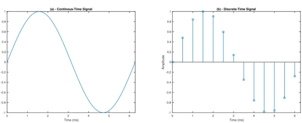
The voltage level is continuous in time, which means some information is lost, during the sampling process (see Figure 2.5). The digital-to-analog is the opposite, it converts the numbers back into electrical voltage.
0 1 2 3 4 5 6 Time (ms) -1 -0.8 -0.6 -0.4 -0.2 0 0.2 0.4 0.6 0.8 1 Amplitude
(a) - Continous-Time Signal
0 1 2 3 4 5 6 Time (ms) -1 -0.8 -0.6 -0.4 -0.2 0 0.2 0.4 0.6 0.8 1 Amplitude (b) - Discrete-Time Signal
Figure 2.5: Signal sampling. When sampling a continous-time signal, some information is lost, only a few points in time are recorded. (a) Continuous signal in time. (b) -Sampled signal.
2.2.2
Nyquist Theorem
The Nyquist theorem, also known as the sampling theorem, is a principle that is fol-lowed in the digitization of analog signals. For a faithful reproduction of the signal, the analog waveform must be sampled frequently. The number of samples per second is called sampling frequency or sampling rate. The most simple case of an analog signal is a sine wave or a sinusoid. These kind of signals have all the energy concentrated
at one frequency. Most signals consist of different components at various frequencies. Bandwidth is defined as a range within a band of frequencies. For analog signals, band-with is expressed in Hertz. The highest frequency component determines the bandband-with of an analog signal. The Nyquist theorem specifies that in order for all the relevant information in an analog signal to be preserved in the sampling process, the sampling rate must be at least 2× Fmax, or twice the highest analog frequency component.
Mathematically, the theorem can be expressed as:
Fs ≥ 2 × Fmax, (2.2)
where Fs is the sampling frequency, and Fmax is the highest frequency contained in the
signal. If a sound wave has a single sine wave at a frequency of 1Hz, the minimum sampling frequency ditacted by the Nyquist theorem is 2Hz. Thus, if this sound wave is sampled at a frequency bigger or equal than 2Hz, there will be more than enough samples on its digitalized version for the human ear to perceive the sound as if it was analogic, and no significant signal information is lost. However, if the signal is sampled at a frequency below than 2Hz, aliasing occurs, because there are not enough samples to capture the significant variations of the signal through time, information will be lost and the result will lead to a different signal being perceived. This is the main reason why industry adopted 44.1 kHz for the CD sampling rate: to cover all the frequencies from the 20 Hz to 20 kHz, which is the highest frequency the human hear can perceive:
44.1kHz > 2× 20kHz (2.3)
2.2.3
Quantization
The sampling process converts a continous-time signal into a discrete-time signal. Each sample or slice, present in the discrete-time signal, contains an amplitude value. The stored amplitude value is the closest to the real one, from a set of possible values. The number of values or levels are expressed in "bits", the binary system. A two bit resolution sampling could store four different values (see Figure 2.6). The most common resolutions are 8-bits, which stores 256 levels, 16-bits, which stores 65536 levels and 32-bits, which stores 4.3 billion levels. The industry adopted 16-bits sampling resolution
for the CD to reproduce a high quality sound.
11
10
01
00
Figure 2.6: 2 bit resolution sampling.
2.3
Music Characteristics
Music is an art resulting from the combination of sounds, that uses rythm, melody, harmony and silence. The Concise Oxford English Dictionary (2002) defines music as:
“the art of combining vocal or instrumental sounds (or both) to produce beauty of form, harmony, and expression of emotion”.
As stated before, sounds are vibrations that travel through the air or another medium. Music sounds have four fundamental characteristics: dynamics, duration, timbre and pitch.
Dynamics
The dynamics of a sound is the perception of the amplitude of the sound wave. This is physically related to the amount of energy that is transported by a sound wave, when the particles vibrate in the medium. It is more commonly referred to as the volume or loudness of a sound. The most common dynamic indications in music, which are also referenced by their Italian words, are very soft (pianissimo), soft (piano), loud (forte) and very loud (fortissimo).
Duration
Each sound occurs during a certain period of time. The duration of a sound is the elapsed time between its start time (onset) and end time (offset).
Timbre
In music, timbre is the quality that distinguishes different types of sounds, e.g. a piano from a guitar. The timbre of a sound is determined by the shape of the sound wave.
Pitch
Is the tonal height of the sound. It is related to how low or how high a note sounds. It is a subjective attribute of sound, that is closely related to the frequency, which is an objective physical property. Pitch is an auditory sensation that maps the vibrations of a sound wave to a tone in a musical scale.
2.4
Signals
Signals can be defined as anything that carries information. Examples of signals are gestures, images, human voice, sounds, etc. Technically, signals can be represented as a function of time, space or other observation variable that transfers information. Audio signals carry a representation of a sound, typically an electrical voltage (see Figure 2.7).
2.4.1
Types of Signals
Signals can be classified in a variety of ways, according to their own characteristics. A brief description will be presented of the characteristics which we find more suitable for the undestanding of this dissertation.
Continuous-Time Signals
A signal is continuous in time if the independent variable (t) is continuous in f (t) and will always have a value. Any analog signal is countinous by nature and analog audio signals are not an exception (see Figure 2.5-a).
0 0.5 1 1.5 2 2.5 3 3.5 4 4.5 Time (ms) -0.05 -0.04 -0.03 -0.02 -0.01 0 0.01 0.02 0.03 0.04 0.05 Amp lit u d e (d b )
Figure 2.7: Sound signal as a function of time.
Discrete-Time Signals
When an analog signal is sampled and converted to bits by an ADC, the signal is represented in small fractions in time. Instead of having a full representation where every instant has a value, we only have a collection of values, depending on the sampling rate and the length of the signal. The signal is represented as x[n], and the independent variable (n) takes on only discrete values (see Figure 2.5-b).
Periodic Signals
A signal is periodic if it repeats itself exactly after some period of time. Some examples of periodic signals are sine waves, square waves, triangle waves, and so on. In continous-time, a signal is periodic if M is an integer and there exists any value T such that:
f (t) = f (t + M T ). (2.4)
The period of the signal is the smallest value of T for which the above relation holds true: the wavelength.
For discrete-time, a signal is periodic if it repeats itself after some period, with one key difference: the period must be an integer. A discrete time signal x[n] is said to be periodic if, both M and N are positive integer values such that:
x[n] = x[n + M N ]. (2.5)
The period of the signal is the smallest value of N for which the above relation holds true.
Quasi-Periodic Signals
Some discrete signals that are almost periodic and can be represented by
x[n]≈ x[n + MN] (2.6)
are called quasi-periodic signals. These signals, when compared to periodic sig-nals, might not have identical points across periods, but will have very similar points. The general waveshape is nearly the same as if it were a periodic signal.
2.4.2
Signal Processing
Signal processing operates in some fashion on a signal in order to extract useful in-formation. It has many application fields, such as audio signal processing, speech signal processing, image processing, wireless communications and so forth. According to the type of signal, signal processing can be divided into five categories: analog signal processing, continuous-time signal processing, discrete-time signal processing, digital signal processing and nonlinear signal processing.
Digital signal processing (DSP) is the manipulation of signals using a general-purpose computer or digital circuits, in order to analyze, filter, create or compress digitalized signals. DSP applications include, among others, digital image processing,
audio signal processing, sonar and radar signal processing, biomedical signal pro-cessing and seismic data propro-cessing. It is applied to digital signals and has also been applied during our work. DSP makes use of several transforms, being the most relevant to our work the Fourier Transform, which will be introduced in the next section.
2.4.3
Fourier Analysis
Regardless of the source of the sound wave, the particles in the air move back and forth at a given frequency. As stated before, the period of the sound wave is the wavelength, and it is also the inverse of the frequency: a sound wave with high frequency will have a smaller period, whereas a sound wave with low frequency will have a larger period (see Figure 2.8). Period
Low Frequency
P
ressur
e
Time
PeriodHigh Frequency
P
ressur
e
Time
Figure 2.8: Low frequency and high frequency representation.
Jean-Baptiste Joseph Fourier had the insight to see that any continuous function could be represented as an infinite sum of oscillating functions. Fourier analysis is the process of decomposing any periodic signal into the sum of a possibly infinite set of sine and cosine functions or complex exponentials. Fourier synthesis is the process of converting those sines and cosines back into a periodic function (see Figure 2.9). A sine wave or sinusoid is a mathematical curve that describes a smooth repetitive oscillation. A sinusoid is represented as a function of time f(t):
y(t) = A× sin(2πft + ϕ) = A × sin($t + ϕ), (2.7)
where A is the amplitude of the wave, f is the number os oscillations per second, 2πf = $ is the angular frequency, and ϕ is the phase.
0 0.2 0.4 0.6 0.8 1 1.2 1.4 1.6 1.8 2
time (in seconds) -1 0 1 1.3 amplitude (a) 0 0.2 0.4 0.6 0.8 1 1.2 1.4 1.6 1.8 2
time (in seconds) -1 0 1 1.3 amplitude (b) 0 0.2 0.4 0.6 0.8 1 1.2 1.4 1.6 1.8 2
time (in seconds) -1 0 1 1.3 amplitude (c) 0 0.2 0.4 0.6 0.8 1 1.2 1.4 1.6 1.8 2
time (in seconds) -1 0 1 1.3 amplitude (d)
Figure 2.9: Figure (a) Approximates the square wave by a sine function with the same F0 (2Hz). Figure (b) represents a sum of two sine waves oscillating at the F0 and an integer multiple of the F0 (called partial). Figure (c) represents a sum of three sine waves oscillating at the F0 and integer multiples of the F0. Figure (d) represents almost a clear decomposition of the square wave into multiple sine functions.
As stated before, a periodic signal can be expressed as a sum of sines or cosines func-tions. In particular, a square wave can be approximated by an odd-multiple frequency sine waves at diminishing amplitude. In Figure 2.9-a, the red curve is described by the
Equation 6.8, and the frequency at which it oscillates is equal to the F0 of the square wave underneath:
y(t) = 1.3sin(2π2t). (2.8)
As we can see in Figure 2.9-b, by summing two sine functions (see Equation 2.9), we can start to see that the result is an approximation of the square wave.
y(t) = 1.3sin(2π2t) + 0.42sin(2π6t). (2.9)
In Figure 2.9-c, we add a third partial (see Equation 2.10), which makes it even closer to the square wave.
y(t) = 1.3sin(2π2t) + 0.42sin(2π6t) + 0.24sin(2π10t). (2.10)
Those multiple sine functions are the frequency components (partials) that make up the composed signal. The frequency of each component or partial is an integer multiple of the fundamental frequency. In Figure 2.9-d, the summation of the sine functions is almost at infinite, reproducing the original signal without almost no difference to the human ear. Each wave oscillates at a specific frequency. The lowest frequency of all waves present in a note is defined as the Fundamental Frequency (F0). Funda-mental frequency is the inverse of the fundaFunda-mental period or P0 and corresponds to the perceived pitch. All the waves are called partials. Frequencies of the partials are mostly limited to integer multiples of the lowest frequency (Fundamental Frequency -F0), forming the harmonic series. A harmonic is a partial that is exactly an integer multiple of F0. F0 is also considered a harmonic partial, because it is one times itself. Except the fundamental frequency, all the partials that make up the harmonic series are called overtones (over F0).
Fourier Series
The Fourier series is used to represent a periodic signal by a discrete sum of complex exponentials. If a continuous function f(t) is periodic with period T, then it may be approximated by a linear combination of harmonically related exponentials. The
Fourier series representation of a periodic signal f(t) is given by the following synthesis equation: ˜ x = ∞ X k=−∞ akejqw0t, k∈ Z, (2.11) where w0 = 2πF 0 = 2π T0
. This equation can be used as a synthesizer to generate a signal as a weighted combination of fundamental frequencies. The corresponding analysis equation for the Fourier series is written as:
˜ ak= 1 T 0 Z T 0 ˜ x(t)ejqw0tdt. (2.12)
The value ak carries the amplitude and the phase of the frequency content of the signal at kw0 Hz. The complex exponentials that form a periodic signal occur only at integer
multiples (harmonics) of the fundamental frequency w0. The synthesis Equation 2.11
can be rearrenged into:
˜ x(t) = a0+ +∞ X k=1 (akejkw0t+ a−ke−jkw0t). (2.13)
If we take into account that a∗k = a−k, furthermore, Equation 2.13 can be expressed as: ˜ x(t) = a0+ +∞ X k=1 (akejkw0t+ a∗ke−jkw0t). (2.14)
The following trigonometric Equation is used to express the Fourier Series of periodic signals and is obtained by reference ak in its polar form as ak=
Ak 2 e jφk: ˜ x(t) = a0+ +∞ X k=1 Akcos(kw0t + φk). (2.15)
A harmonic sound is a periodic signal and can be represented by Equation 2.15. Quasi-periodic signals do not have frequencies at multiple locations of its fundamental fre-quency. Those frequencies are simply referred to as partials, instead of harmonic partials, since their frequency is not an exact multiple of the corresponding F0. For an approximation of this type of signals, a finite number of harmonic components H is used: ˜ x(t)≈ a0+ H X k=1 Akcos(kw0t + φk). (2.16) Fourier Transform - FT
The Fourier transform (FT) is used to represent a periodic signal (function) by a countinous superposition or integral of complex exponentials. It decomposes a signal as a function of time into multiple frequencies resulting in a complex-valued function of frequency. The absolute value represents the frequency band over a range of frequencies present in the original signal and the complex value represents the phase offset of the sinusoid in that frequency. The FT is generally used in signal processing, specially in time-frequency analysis. For a periodic signal, with infinte length, it is defined as:
F Tx˜(f ) = ˜X(f ) =
Z +∞ −∞
˜
x(t)e−j2πf tdt. (2.17)
This equation results in the frequency domain representation of the original signal.
Discrete Fourier Transform - DFT
The Discrete Fourier Transform (DFT) is the equivalent of the continuous Fourier Transform for sampled signals. The DFT is used to perform Fourier analysis in many practical applications, such as digital signal processing. DFT can be achieved in a continous sampled signal by applying the following equation:
DF T˜x[k] = ˜X[k] = +∞ X n=−∞ ˜ x[n]e−j2πkn, (2.18)
an infinite continous-sampled signal is not efficiently possible, one must restrict the size of the signal. Having N as number of samples, the DFT for finite signals is represented as: DF Tx˜[k] = ˜X[k] = N −1X n=0 ˜ x[n]e−j 2π N kn, k = 0,· · · , N − 1. (2.19)
The magnitude spectrum (see Figure 2.10) is given by| ˜X[k]|.
The problem with DFT is that it requires 2N2 real multiplications and additions, which makes it really hard to apply in real-time signal processing.
Fast Fourier Transform - FFT
The Fast Fourier Transform (FFT) is an algorithm which optimizes the DFT and was invented by Gauss in 1805, and later re-discovered by Cooley and Tukey in 1965. The FFT applies to signals that have a structured number of samples, such as a power of 2. The first step of the FFT is to decompose an N point time-domain signal into N time domain-signals, where each signal is composed of a single point. Then, the frequency spectra of each N time-domain signals are computed. The last step is to aggregate and synthesize all the N spectra into one single frequency spectrum. Through this method, the FFT only requires N log2N operations, which allows its application in real-time
signal processing.
2.4.4
Power Spectral Density
Power Spectral Density function (PSD) represents the strength of variations as a func-tion of frequency and is computed from the squared magnitude value of the DFT of a signal. The unit of PSD is energy per frequency. The PSD is obtained by applying | ˜X[k]|2, assuming that ˜X[k] is the DFT of a signal x[n]. By integrating PSD within a specific frequency range, we obtain the energy for those frequencies. The result of the DSP application is the power spectrum (see Figure 2.11).
0 100 200 300 400 500 Frequency (Hz) 0 5 10 15 20 25 30 35 40 Amplitude 23.25 31 46.5 92 Time (ms) -0.15 -0.1 -0.05 0 0.05 0.1 Amplitude
Figure 2.10: The left image shows the signal x(t) in time, whereas the right image shows the magnitude spectrum or absolute value of the DFT - | ˜X[k]|.
0 1076 2152 3228 4304 Frequency (Hz) 0 5 10 15 20 25 30 Amplitude
(a) - Magnitude Spectrum
0 1076 2152 3228 4304 Frequency (Hz) 0 200 400 600 800 Amplitude
(b) - Power Spectral Density
Figure 2.11: This figure compares the magnitude spectrum given by | ˜X[k]|, and the Power Spectral Density given by| ˜X[k]|2.
2.4.5
Spectral Leakage
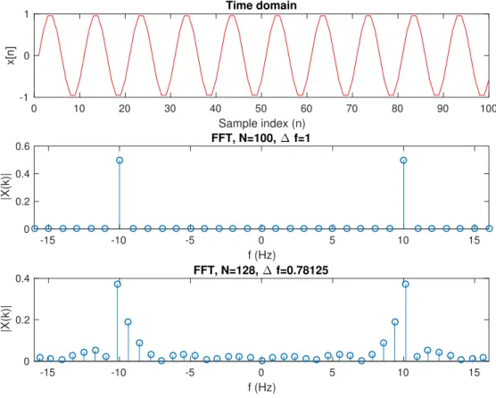
The DFT assumes that the input repeats over and over again (periodic). If a sinewave oscilates at 10 Hz, we would have to calculate the number of samples to work on, to give us the exact period. If the DFT is applied to a signal that is not periodic (the number of samples do not finish on a whole number of periods), discontinuity will occur, and the frequency representation of the signal will be distorted (see Figure 2.12). An effect known as spectral leakage occurs when the energy of a frequency bin is leaked or spread across adjacent frequency bins. This effect could interfere with the overall shape of the magnitude spectrum.
0 10 20 30 40 50 60 70 80 90 100 Sample index (n) -1 0 1 x[n] Time domain -15 -10 -5 0 5 10 15 f (Hz) 0 0.2 0.4 0.6 |X(k)| FFT, N=100, ∆ f=1 -15 -10 -5 0 5 10 15 f (Hz) 0 0.2 0.4 |X(k)| FFT, N=128, ∆ f=0.78125
Figure 2.12: The top chart displays a 10hz sinewave, sampled at a 100hz sampling rate. The middle chart displays the DFT applied to the 100 samples of the signal, a whole number of periods. The bottom chart displays a spectral leakage, because the DFT was applied to more samples than the period.
2.4.6
Windowing
In order to minimize the spectral leakage effect, the samples in the frame can be multiplied by a smooth window shape. This will smooth the abrupt edges caused by the truncation of a signal into a single time window. Windowing is the process where the input time signal is multiplied by a windowing function (see Figure 2.13). This process is often used for spectral analysis, filter design, and beamforming. When we want to apply the FFT to a signal, we have to choose which interval do we want to analyse. There are multiple types of windows: triangular, Parzen, Hanning, Hamming, Blackman, and so on.
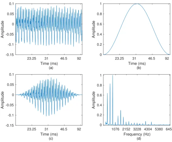
23.25 31 46.5 92 Time (ms) -0.15 -0.1 -0.05 0 0.05 0.1 Amplitude (a) 23.25 31 46.5 92 Time (ms) 0 0.2 0.4 0.6 0.8 1 Amplitude (b) 23.25 31 46.5 92 Time (ms) -0.15 -0.1 -0.05 0 0.05 0.1 Amplitude (c) 1076 2152 3228 4304 5380 6456 Frequency (Hz) 0 0.2 0.4 0.6 0.8 1 Amplitude (d)
Figure 2.13: Preprocessing process: (a) input time signal piano note, (b) Hanning window, (c) resulting windowed signal, (c) frequency domain signal.
2.4.7
Relation between the signal’s properties
It is important to distinguish both time resolution and frequency resolution and the implications that both have in signal analysis. The number of samples of a signal varies with the sampling rate and the seconds of information that we have. Having Fs as the
sampling rate and t as the number of seconds recorded, we can calculate n, the total number of samples recorded:
n = Fs× t (2.20)
is also discrete, being k the corresponding Frequency Bin. This way, by analyzing Equation 2.19, we can see that the frequency resolution is related to the number of samples (N ). Thus, frequency resolution is the distance in Hz between two adjacent frequency bins in the DFT and can be expressed as:
∆F = Fs
N, (2.21)
where N is the DFT window size.
Time resolution, on the other hand, is the minimum time of a signal in seconds that one could extract information from.
∆t = N Fs
. (2.22)
If we have a 2 second music signal recorded at a sampling rate of 22050 samples per second, we would end up with 22050×2 = 44100 samples. Let us consider that the DFT has a window size of 4096 samples. The frequency resolution is 22050
4096 , which means that each bin, will correspond, approximately, to 5,38 Hz. The time resolution is 4096
22050, which means that we could only detect musical notes with duration equal or greater then 0.19 seconds. The window size of the DFT must be properly set according to the type of information that we want to focus on, either time information or frequency information. The greater the DFT size is, the shorter the frequency resolution is, which makes it easier to analyse low frequencies, but it will increase the time resolution, which makes harder to analyse shorter periods of time.
2.4.8
Missing Fundamentals
A missing fundamental occurs when we perceive a fundamental frequency in a sound, that does not have that frequency. The missing fundamental or phantom fundamental, may be created by the overtones present in the signal such that, together, suggest a frequency that does not exist. The brain perceives a pitch by the fundamental frequency or the periodicity of an audio signal. If a signal has two pure tones at 1000 Hz and 1300 Hz, we might perceive a missing fundamental by hearing those two frequencies and an additional one, created by the difference of the two signals. We would end up
with one additional pitch correspondent to the frequency of 300 Hz, because of the form of the waveform (see Figure 2.14).
0 0.005 0.01 0.015 0.02 0.025 time (msec) -1 0 1 amplitude Pure tone of 1000 Hz 0 0.005 0.01 0.015 0.02 0.025 time (msec) -1 0 1 amplitude Pure tone of 1300 Hz 0 0.005 0.01 0.015 0.02 0.025 time (msec) -2 0 2 amplitude
Complex tone: 1000 Hz + 1300 Hz pure tones
Figure 2.14: Complex tone with a phantom frequency at 300Hz.
2.4.9
Pitch
Each musical note is composed by an harmonic series: its fundamental frequency (F0) and the corresponding partials. What the human ear perceives as Pitch is the fun-damental frequency (i.e.: lowest harmonic partial) of each harmonic series or musical note. A sound wave that vibrates at a specific frequency, will be mapped internally by our brain to a certain pitch. Each pitch is related to a musical note (see Figure 2.15). If, for instance, we hear a sound wave vibrating at, approximately, 262 Hz, our brain will map internally that sound wave to the pitch C4 (middle C in a 88 keys keyboard), because the fundamental frequency of C4 is, approximately, 262 Hz. Since pitch is
an auditory sensation, if the previous sound wave vibrates at 260 Hz or 262 Hz, our brain probably would still map it to a C4 pitch. One octave higher (pitch C5) has the fundamental frequency of, approximately, 523 Hz. Comparing this two signals, pitch C5 will sound ’higher’ than pitch C4. The distance perceived between C2 and C3 (66 Hz) is the same as the distance between C3 and C4 (131 Hz), since the human ear perceives pitch in a logarithmic scale: for each octave, the frequency doubles. Note that A2, A3, A4 and A5 have 110Hz, 220Hz, 440Hz and 880Hz respectively.
NOTE
OCTAVE
0 1 2 3 4 5 6 7 8
16 33 65 131 262 523 1047 2093 4186 17 35 69 139 278 554 1109 2218 4435 18 37 73 147 294 587 1175 2349 4699 20 39 78 156 311 622 1245 2489 4978 21 41 82 165 330 659 1319 2637 5274 22 44 87 175 349 699 1397 2794 5588 23 46 93 185 370 740 1475 2960 5920 26 52 104 208 415 831 1661 3322 6645 29 58 117 233 466 932 1865 3729 7459 25 49 98 196 392 784 1568 3136 6272 28 55 110 220 440 880 1760 3520 7040 31 62 124 247 494 988 1976 3951 7902 C C# D D# E F F# G G# A A# BFigure 2.15: Pitch to frequency relationship. C4 has the frequency of 262 Hz.
2.4.10
Pitch vs Fundamental Frequency
Pitch detection and F0 detection are two different processes that are easily confused. Several algorithms have been developed to address the single-pitch and multi-pitch estimation problems. In the overall, what all try to achieve is the pitch transcription,
what notes are being played. Fundamental frequency estimation approaches, try to identify exactly the frequency of the signals. After knowing which F0 or F0s are present in the signal, they are mapped to pitches or notes. Pitch estimation approaches, try to identify the pitch or pitches present in the signal, without the need of knowing exactly what is the exact fundamental frequency. In this dissertation, the problem which we are trying to solve is the pitch estimation, not the fundamental frequency estimation.
2.5
Single-Pitch Estimation
Signals where several sounds are played simultaneously are called polyphonic signals, in contrast to monophonic signals, where at most one note is present at a time (Klapuri and Davy, 2006). Yeh (2008) states that, without loss of generality, a monophonic signal can be expressed as a sum of a quasi-periodic part ˜x[n] and the residual z[n]:
x[n] = ˜x[n] + z[n]≈
H
X
h=1
Ahcos(hω0n + φh) + z[n]. (2.23)
The goal is to extract the periodicity part of x[n], and not to minimize the residual z[n]. The most common errors are harmonically related to the correct F0: subharmonic errors and super-harmonic errors. Subharmonic errors are errors in which the results are unit fractions of the correct F0 and super-harmonic errors are errors in which the results are multiples of the correct F0. Single-F0 estimation algorithms can be classified as time domain approaches or spectral domain approaches. Temporal domain methods try to find the fundamental period, as opposed to frequency-domain methods which rely on the spectral analysis.
2.5.1
Spectral-location Approaches
Time domain methods look for a similar repetitive waveform in x[t] through pattern matching between x[t] and a delayed version of x[t]. Pattern matching in time domain can be carried out through multiplication or subtraction between patterns.
2.5.1.1 Autocorrelation
The autocorrelation function (ACF) allows to measure the similarity between a sig-nal and delayed versions of itself at different points in time. It corresponds to the cross-correlation of a signal with itself for a given lag or delay. Mathematically, the autocorrelation function can be calculated as the sum of the product between a signal x[n] of finite duration L and its delayed version x[n + τ ], for each lag τ :
ACF [τ ] = 1 L
L−τ −1X
n=0
x[n]x[n + τ ]. (2.24)
For quasi-peridic signals, correlation will be higher when τ equals the period or a multiple of the period. Nonetheless, this technique is sensitive to resonance in music signals.
2.5.1.2 Magnitude difference
Ross et al. (1974) evaluate the distance between two patterns by comparing the dissimi-rality of x[n] and x[n+τ ]. This method is called the Average Magnitude Difference Function (AMDF). It is used often for real time applications as it involves less com-putation. Analytically, it is represented by:
AM DF [τ ] = 1 L− τ
L−τ −1X
n=0
|x[n] − x[n + τ]|. (2.25)
For quasi-periodic signals, the result of the AMDF is particularly small at delays cor-responding to the period or integer multiples of the period. The AMDF is not very accurate when the signal has background noise. Ghulam (2011) extended this tech-nique to address this issue. A similar techtech-nique called Squared Difference Function (SDF) measures the dissimilarity by the squared difference:
SDF [τ ] = 1 L− τ
L−τ −1X
n=0
(x[n]− x[n + τ])2. (2.26)
normalizing SDF with its average over shorter-lag values. It is commonly addressed as Cumulative Mean Normalized Difference Function and avoids super-harmonic errors. Both methods are related to the autocorrelation function. Hess (1983) demon-strated that both those methods are error prone when submited to intensity variations, noise and low-frequency spurious signals.
2.5.1.3 Cepstrum
The cepstrum is the result of taking the Fourier Transform (FT) of the logarithm of the power spectrum of a signal. This results in a complex cepstrum, a real cepstrum, a power cepstrum and a phase cepstrum. This technique is useful to measure the periodicity between peaks in the frequency domain. The real cepstrum or the power cepstrum is calculated by applying the following equation:
c(τ ) = IDF T{log |DF T (x[n])|)}. (2.27)
Schroeder, in 1962, proposed the application of the power cepstrum for F0 estimation based on the first cepstral analysis paper on echoes resulting from earthquakes and bomb explosions. Noll (1967) proposed, later, a short-time power cepstrum analysis for pitch determination of human speech. The spectral envelope information if given by the lower-quefrency components in the cepstrum. The period candidates correspond to the sharp cepstral peaks components.
Figure 2.16 shows three time-domain salience functions applied to a baritone sax signal of T 0 = 2.3ms.
2.5.2
Spectral-interval Approaches
In spectral domain approaches, F0 estimation is performed by extracting the period-icity from the spectrum, after applying a Fourier Transform. The resulting spectrum contains the spectral information of the harmonic, including its partials at almost in-teger multiples of the fundamental frequency. One approach of the spectral domain techniques is to measure the space between dominant peaks and assume it as the F0 of the signal. Another approach is to extract the F0 based on a function of hypothetical partials. Based on this assumptions, Yeh (2008) states that fundamental frequency can
0 2 4 6 8 10 12 −0.5 0 0.5 time (msec) Waveform (A) 0 2 4 6 8 10 12 −0.05 0 0.05 0.1 ACF (B) 0 2 4 6 8 10 12 0 0.1 0.2 0.3 0.4 AMDF (C) 0 2 4 6 8 10 12 0 0.1 0.2 0.3 SDF (D) 0 2 4 6 8 10 12 0 1 2 Cepstrum (E) lag (msec)
Figure 2.16: (A) signal waveform; (B) autocorrelation function; (C) average magnitude difference function; (D) squared difference function; and (E) cepstrum. Figure taken from Reis (2012), page 26, with permission.
also be defined as the greatest common divisor of the frequencies of all the harmon-ics.
2.5.2.1 Spectral Autocorrelation
Lahat et al. (1987) showed that since the autocorrelation function searches for repet-itive patterns in the time domain, it can also be applied to the spectral domain. The periodicity is obtained by pattern matching between the spectrum and its shifted ver-sions. The ACF function applied to the magnitude spectrum is calculated as:
ACF S(m) = 2 K− 2m k 2X−m−1 k=0 |X[k]||X[k + m]|, (2.28)
m is equal to F0, the ACFS should result in the maximal spectral autocorrelation coefficient. The product between the spectrum and the shifted spectrum is attenuated when the shift m is not equal to F0 or multiples of F0, since the partial peaks are not aligned.
2.5.2.2 Harmonic Matching
Harmonic matching or pattern matching makes use of harmonic spectral patterns to match the observed spectrum. These harmonic spectral patterns can either be a spe-cific spectral model or a harmonic comb without specifying the amplitudes of the harmonics. A harmonic comb is a series of spectral pulses with equal spacing defined by a F0 hypothesis. Specific spectral models are often used in multi-pitch signals, whereas harmonic comb is often used on single-pitch estimation. In the works of (Martin, 1982) and (Brown, 1992), a F0 hypothesis can be evaluated based on the correlation between the harmonic comb and the observed spectrum. In Goldstein (1973) and Duifhuis and Willems (1973) a F0 hypothesis is evaluated based on the minimization of the dis-tance between the frequencies of the harmonics and the frequencies of the matched peaks.
2.6
Multi-Pitch Estimation
Multi-pitch estimation algorithms are used for short-time signals that can have more than 1 harmonic source at the same time. Yeh (2008) stated that those signals can be expressed as a sum of harmonic sources Ym[n] plus a residual z[n], where M is the
number of harmonic sources:
y[n] =
M
X
m=1
Ym[n] + z[n], M > 0. (2.29)
The goal of multiple-F0 estimation algorithms is to infer the number of sources and the related F0s. The residual z[n] is not related to the sinusoids but can be explained by background noise, spurious components or inharmonic partials. Equation 2.30 rep-resents this model by the Fourier Series.
y[n] = M X m=1 { ∞ X k=1 Am,kcos(kωmn + φm,k)}. (2.30)
The complexity of polyphonic music signals is far superior to monophonic music sig-nals.
Figure 2.17: Comparison between two spectrograms of monophonic and polyphonic signals. 1 2 3 4 5 6 7 8 9 10 Time (mins) 0 0.05 0.1 0.15 0.2 0.25 0.3 0.35 0.4 0.45 0.5 Normalized Frequency ( × π rad/sample) -110 -100 -90 -80 -70 -60 -50 -40 -30 -20 Power/frequency (dB/rad/sample)
(a) Spectrogram of a monophonic signal, recorded from a piano.
1 2 3 4 5 6 7 8 9 10 Time (mins) 0 0.05 0.1 0.15 0.2 0.25 0.3 0.35 0.4 0.45 0.5 Normalized Frequency ( × π rad/sample) -120 -110 -100 -90 -80 -70 -60 -50 -40 -30 -20 Power/frequency (dB/rad/sample)
(b) Spectrogram of a polyphonic signal, recorded from a piano.
Figure 2.17a shows the representation of a spectrogram of a monophonic signal, recorded from a piano and Figure 2.17b is the representation of a spectrogram of a polyphonic signal with 4 harmonic sources, recorded from a piano. As we can see, the spectrogram of a polyphonic signal has more frequency components than a monophonic signal. In polyphonic music we need to infer the number of harmonic sources, whereas in mono-phonic music there is no such need, because we only deal with one harmonic source. Extracting the correct multiple F0s from a music piece is very difficult, due to the overlapping partials, transients, reverberation and the different spectral characteristics of the musical instruments.
2.6.1
Overlapping Partials
For polyphonic signals, different harmonic sources may overlap or interfere with one another, in time and in frequency. Different sources, in polyphonic signals, with funda-mental frequencies Fa and Fb are harmonically related when they can be represented
by Equation 2.31.
Fa=
m
nFb, n, m∈ N. (2.31)
As demonstraded by Klapuri (1998), every nthpartial of the source a overlaps every mth partial of source b. This frequently happens when the sources are harmonically related to each other, since it could result in partial colisions. One of the issues when dealing with multi-pitch signals is that most of the musical notes are harmonically related, which results in a high probability of partial overlapping. Another issue is that when fundamental frequencies of two notes are multiples of each other, the partials of the higher note may overlap completely with those of the lower note (Yeh, 2008). The frequencies, amplitudes and phases of the overlapping partials of harmonic sources are thus disturbed. Parsons (1976) addressed the problem of separating the voice of a vocalist speech, by trying to detect the overlapping components, based on three tests: spectral peak symmetry, distance and well-behaved phase. This technique is restricted to two voices and relied on the sinusoidality of stationary sinusoids and is not suitable for modulated sinusoids. As highlighted by several authors, it still remains very difficult to decompose the overlapping partials into their original sources, even if the number of concurrent sources is known beforehand (H. Viste and G. Evangelista (2002);Virtanen (2003);Every and Szymanski (2004);Yeh and Roebel (2009)).
2.6.2
Spectral Characteristics
Since polyphonic music signals could have multiple instruments playing at the same time, the diverse spectral characteristics of each one, increases the complexity of the transcription problem.
2.6.2.1 Spectral Envelopes
Spectral envelope denotes a countour that passes through the peaks of the spectrum. Generally, those peaks are the partials of the signal. Many musical instruments have smooth spectral envelopes but differ immensely in their shapes. The spectral shape also evolves with time, by having partials decaying at different rates. Furthermore, pianos, bassoons, oboes and guitars often produce relatively weak fundamentals on the lower frequencies. A universal model that generalizes musical instruments still has to be developed, according to previous studies (Jensen (1999); Loureiro et al. (2004); Burred et al. (2006)).
2.6.2.2 Inharmonic Partials
Because of the physical properties of instruments, most of them do not produce sounds with harmonic partials, but partials slightly deviated from the ideal frequency. Those partials are called inharmonic partials, and occur often in string instrument sounds. The measure of how much inharmonic partials are deviated from their ideal frequencies, is called inharmonicity deviation. For strectched strings, the frequencies of the partials are given by the Equation 2.32, where F is the fundamental frequency, h is the partial number, and β is the inharmonicity factor (Fletcher and Rossing, 2008).
fh = hFp1 + β(h2− 1), (2.32)
A harmonic model needs to allow for certain inharmonicity in order to explain the frequency deviation from each partial. If that is not the case, additional sources may be needed to explain the inharmonic partials.
2.6.2.3 Spurious components
Some instruments have dominant frequency components excited along with the partials, called phantom partials. These phantom partials, observed in string instruments, are related to the tension variation of the plucked strings and appear close to the frequencies of the partials (Conklin, 1999).
2.6.3
Transients
Transients can be simply stated as an event or zone of short duration where a fast variation of the sound signal occurs (Rodet and Jaillet, 2001). These variations can occur at note onsets as fast attacks or at note offsets with fast releases. Due to its highly non-stationary nature, it is very difficult to estimate the correct F0 within transients. As demonstrated by McIntyre et al. (1983), sometimes the attack transient also excites subharmonics on bowed and woodwind instruments. Transients often have high energy which results in spectral collisions with other sound sources. Recent research deal with transients as a specific signal component. Rodet and Jaillet (2001), Röbel (2003) and Bello et al. (2005) detect transients by applying non-parametric approaches, as oposed to Molla and Torrésani (2004) and Daudet (2004), which applied parametric approaches.
2.6.4
Reverberation
Reverberation prolongs preceding sounds by overlapping them with the following sounds, and also increases the complexity of the task of F0 estimation. A recorded signal be-comes a mixture of multiple sounds, such as direct sounds, reflected sounds and rever-berated sounds. As studied by Beauchamp et al. (1993), Baskind and De Cheveigné (2003) and Röbel et al. (2006), even a record of a monodic instrument in a reverber-ant environment can be polyphonic. The reverberated parts are often non-stationary, adding even more complexity to the analysis of the signal.


![Figure 2.10: The left image shows the signal x(t) in time, whereas the right image shows the magnitude spectrum or absolute value of the DFT - | X[k]˜ | .](https://thumb-eu.123doks.com/thumbv2/123dok_br/18547484.905710/42.892.145.708.376.839/figure-image-shows-signal-right-magnitude-spectrum-absolute.webp)
![Figure 2.11: This figure compares the magnitude spectrum given by | X[k] ˜ | , and the Power Spectral Density given by | X[k]˜ | 2 .](https://thumb-eu.123doks.com/thumbv2/123dok_br/18547484.905710/43.892.173.742.191.649/figure-figure-compares-magnitude-spectrum-power-spectral-density.webp)