Abstract— Researchers have always been in face of path loss

(1)

Brazilian Microwave and Optoelectronics Society-SBMO received 26 Jan 2018; for review 09 Feb 2018; accepted 16Aug 2018 Brazilian Society of Electromagnetism-SBMag © 2018 SBMO/SBMag ISSN 2179-1074

Abstract—_{Researchers have always been in face of path loss}

calculation in different media for applications such as telecommunication link design. Wave propagation calculations in large spaces using the FDTD method is time-consuming and imposes a great computational burden. For this reason, to replace the classical FDTD method for wave propagation simulation and path loss calculation in large spaces, optimized methods, namely TDWP, have been provided. In this paper, the use of the TDWP method for wave propagation simulation and path loss calculation above a terrain is investigated. Longitudinal components of ground-waves are taken into account (including direct waves, ground reflections, and surface waves). Propagation space is longitudinally divided into smaller FDTD windows with finite length. The electromagnetic pulse travels through these windows from left to right to the desired point. But despite its capability in reducing computational burden and increasing processing speed, TDWP has lower precision in instantaneous field simulation and calculation of propagation coefficients, so that results obtained from FDTD and TDWP are clearly different. In this paper, some efficient methods are proposed, which yield an increase in method accuracy.

Index Terms— _{Electromagnetic wave propagation, Groundwaves, Surface} wave propagation, Terrain modeling, Consecutive windows, Finite-difference time-domain (FDTD), Time-domain wave propagation (TDWP)

I. INTRODUCTION

Modern communication and radar systems need effective tools to foresee propagation. In many cellular communication and HF and VHF radar sites, high precision propagation simulation is vital. The results are necessary for choosing proper places for ground stations and optimum height for transmitters and receivers, and also reducing the costs of implementing communication systems. One

of the primary aims of propagation simulation is to forecast path loss ( ) with high precision. Path loss is defined as:

Comparison of FDTD and TDWP Methods

for Simulating Electromagnetic Wave

Propagation above Terrains

Mahmoud Fallah

,

Amir. H Nazeri

,

(2)

T T R P

R S

P G G

L

P L



(1)

Where , , , , , and denote transmitted power, transmitter antenna gain, receiver antenna gain, propagation loss, and system loss, respectively. In (1), antenna gains are measured with respect to an isotropic reference antenna, and represents all system losses, including thermal loss, signal loss in cables, mismatch loss, etc. For example, this equation is used in cellular communication system design to foresee each antenna coverage and dead zones before they are installed. Propagation loss denotes all loss caused by factors such as propagation medium refraction index, multipath interference, and reflections from natural and man-made obstacles. So the simulator must take all such parameters into account.

In the past two decades, researchers have been in favor of path loss calculation, with numerous efforts made in this direction. In [3], virtual tools for ground-wave propagation modeling and numerical simulation strategies are reviewed. The propagation loss of 71 floors in 17 different buildings, in an urban area, is measured in 4 frequencies ranging from 800 MHz to 8 GHz in [4]. In [5], a study of path loss models in the 2 – 73.5 GHz range in an Urban-Macro Environment is performed. In [6], electromagnetic (EM) wave measurement in 2.4 GHz in underwater environment is conducted. Also, it is shown that the propagation velocity and absorption coefficient in fresh water are frequency independent.

So far, several numerical methods have been introduced for the analysis of electromagnetic problems. Most of these methods are based on full-wave analysis in the time or frequency domain; and utilize one or two difference equations, plus boundary conditions (depending on the specific case) to solve the problem [7 – 10]. Each method is used to solve a specific class of problems. Although these methods are powerful and can be used to solve a wide variety of problems, due to improper usage and intrinsic limitations, sometimes the derived answer is erroneous. Unless errors such as overflow or underflow have occurred, computers always produce answers. The case is whether this answer correctly represents the physics of the problem in the real world.

One of the most ubiquitous methods is the finite-difference time domain, or FDTD method for short. This method is performed in the time domain and has been used for decades. Although real wave propagation takes place in three-dimensional space, a two-dimensional FDTD approximation can be used, if the problem is symmetric relative to one of the coordinate axes.

(3)

Brazilian Microwave and Optoelectronics Society-SBMO received 26 Jan 2018; for review 09 Feb 2018; accepted 16Aug 2018 Brazilian Society of Electromagnetism-SBMag © 2018 SBMO/SBMag ISSN 2179-1074 performed using both TWDP and FDTD, and the results are compared. Finally, the simulation process is modified to reduce these differences.

II. TDWPMETHOD

The wave propagation problem may be set in city streets with numerous buildings, in a vast desert, or in a mountainous area. The classical FDTD method faces shortcomings when simulating wave propagation along long paths. Suppose we would like to study wave front propagation with spatial Gaussian distribution (along the height axis) in a 10 km path and a height of 50 m. If we divide this space into a mesh of 10 cm cubic cells, there would be 5000000 cells in this space, not considering PML blocks located at the left, right, and top of the computational space. The propagated wave consists of three components, regardless of its polarization. Every time these three components are updated, the new values should be stored in matrices. So we need three matrices with 5 milli

on elements each, all with 15 million elements updated in every time step. Considering the fact that

the utilized program uses some of the computer’s RAM and CPU cycles, it can be concluded that

processing such huge amounts of data with personal computers is impossible. Even if sufficient RAM capacity is obtained, processing the data takes considerable time.

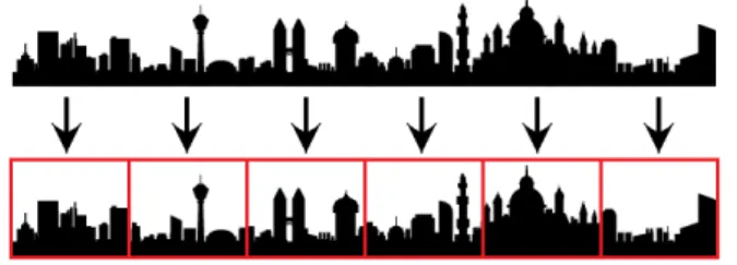
To overcome this problem, instead of updating all components for every computational cell at every moment, a rectangular window around the pulse can be presumed, containing most of the propagated pulse energy. In this manner, the computational space can be divided into smaller windows, as shown in fig. 1 and 2.

Fig 1. Dividing natural terrain into smaller computational regions

Fig 2. Dividing urban terrain into smaller computational regions

These smaller rectangular windows must be surrounded by PML from the left, right, and top. PML blocks surrounding the computational space prevent reflection and refraction of the waves along the

boundaries. The aim is to compute propagation loss along the wave’s path and also along the height

(4)

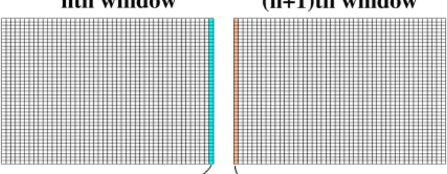
Brazilian Microwave and Optoelectronics Society-SBMO received 26 Jan 2018; for review 09 Feb 2018; accepted 16Aug 2018 Brazilian Society of Electromagnetism-SBMag © 2018 SBMO/SBMag ISSN 2179-1074 adjacent cells, the wave front begins to move along the length of the window to its border. When the wave front first reaches the last column of cells in this window, the magnitude of field components in this column are stored in some part of the computer memory, until the effective pulse energy reaches the end of the current window. After the resulting data is stored, the first window is closed and a new computational space is defined as the second window, containing the physical properties of the next compartment. In the new window, all cell field components are initially zero, which means that none of the cells are stimulated. The field components of cells in the last column of the preceding window are immediately copied as field components of cells of the first column of the current window (fig.3). Similar to the first window, the pulse travels to the second window, and the same procedure is repeated. By continuing in the same manner for numerous windows, pulse flight can be simulated for paths as long as tens of km.

Fig 3. Storing and restoring field components in two consequent windows

In fact, in this manner, a rectangular computational space with very great length is divided into rectangular computational spaces with smaller length, but the same height as the huge rectangle, so that the simulation can be readily done with a personal computer.

III. PROBLEM FORMULATION

A. Wave Propagation Formulation

Although the physics of propagation is taking place in a three-dimensional space, for a symmetrical problem with respect to one of the Cartesian coordinates, we can use a two-dimensional FDTD

approximation. Maxwell’s equations and the constitutive parameters, in the form of vector differentials, in an isotropic space containing magnetic and dielectric materials, are as follows:

(n+1)th window nth window

Cells of the first column of the (n+1)th window, where field components of the last column of the preceding window are restored. Cells of the last column of

(5)

* * . . B E H t D H E t D B                     

(2) r

r

B H H

D E E

  

  

 

  (3)

Where

B



and

D



are associated to the

H



and

E



vectors.



And



* are the electric and magnetic

conductivity of the material, and



and



* are the electric and magnetic charge, respectively. By

assuming

TM

y



Hy,Ex,Ez



polarization for the propagated wave and considering a zero value for the electric and magnetic conductivity coefficient, equation 2 and 3 can be simplified as:

(

4 )

y _z _x

H E E

t x z

        

(

5 )

y z H E t x      

(

6 )

y x H E t z       

(6)

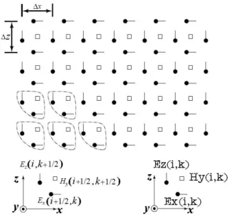
Fig 4. Configuration of the nodes of electric and magnetic fields for TM polarization used in simulation

With the above explanations, and assuming a discrete time form of ₁ 2 1 2 n n

t

 







_

_







, equations 4, 5 and 6 can be indexed:

(

7 )

 





 

















1 1

2 _, 2 _,

1, ,

, 1 ,

n n y y n n z z n n x x

H i k H i k

t

E i k E i k x

t

E i k E i k z               

(

8 )

 

1

 

1₂

 

1₂





, , , 1,

n z

n n

n

z y y

t

E i k E i k H i k H i k

x          













(

9 )

 

1

 

1₂

 

1₂





, , n , n , 1

n n

x x y y

t

E i k E i k H i k H i k

z          













The components of the electric and magnetic field are calculated in the t, 2t , 3t , , n t ,

and 1 , 3 , 5 , , 1

2t 2 t 2t n2 t

 

 

  moments, respectively.

(7)

IV. PATH LOSS CALCULATION

In this problem, the propagation space is a semi-confined space, limited by and

vertically, and by and in the plane parallel to the ground. We would like to calculate the loss caused by the propagation medium, without considering the effect of the receiver and transmitter antenna. In other words, we would like to calculate the power lost in propagation, after the wave is transmitted by the transmitter antenna, before it is absorbed by the receiving antenna. Therefore, in (10), , , and should be substituted with 1. In every given point, can be calculated in terms of field magnitude [2]:

(10)

Therefore, to compute the propagation loss, we need to calculate the electric field magnitude at every given point in the propagation space.

(8)

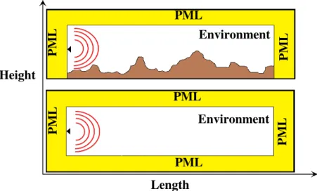
Fig 5. For every scenario, two simulation steps should be performed. In the first, the fields are calculated in the presence of the terrain. In the second, the fields are calculated without regarding the terrain.

Finally, after both steps are done, by performing DFT analysis on the time-domain data available (in the desired bandwidth), for each desired frequency is derived. Usually, it would be favorable

to calculate and plot this ratio in decibel units (2* ) for a specific distance or height.

A. Source Stimulation

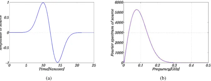
To stimulate the fields of the computational space, we need to model a physical source. Because finite time distributions, which also have limited frequency bandwidth, provide better responses in FDTD simulations, the pulse shape (in the time domain) is usually selected as Gaussian. However, here we prefer to use the derivative of the Gaussian function, in order to prevent DC effects that can cause shifting of the wave propagation frequency in some applications. However, we should note that the desired pulse for our source should cover the range of frequencies determined by the bandwidth. The Gaussian function derivative used in our algorithm is as follows:

(

11 )







 2



2

( )

2 / 3

4 2 / 74

,

t

f t

t

e

BW

 











 

 





Where  is the time shift of the function toward the positive direction of the time axis; which is equal

to

4 

in our case. The pulse shape of the Gaussian function derivative in the time and frequency

domains are given in fig. 6, respectively, forBW 200 MHz.

Height

Length

Environment

PML

PM

L

PM

L

PML

PM

L

PM

(9)

(a) (b)

Fig 6. a) The diagram of the Gaussian pulse derivative in terms of time for the bandwidth 200MHz , b) The diagram of the Fourier transform of the derivative Gaussian pulse.

Now which

i

and

j

the simulation applies to depend on the type of stimulation. The distribution, e.g.

pulse time distribution, can also be in different forms. One of the most popular spatial distributions

along the vertical axis is the Gaussian distribution; where its centricity is shown with

h

_

source

.

The statistical process of spatially distributing the pulse along the

z

axis is achieved by its variance

.

2

1 ( _ )

( ) exp

2

2 v v

z h source G z

 

 





_



_





(12)

source

h

_

is the height of the spatial distribution center for the source from the ground and



_v is the spatial variance of the source. In fig.7, the spatial distribution of the source with centricity of

m source

h_ 25 from the ground at a height of 50 m is shown for different variances.

Fig 7. Spatial distribution of the source with centricity of Z₀ 25mfrom the ground at a height of 50 m for different variances

(10)

(

13 )

)

(

)

(

)

,

(

z

t

G

z

F

t

pulse



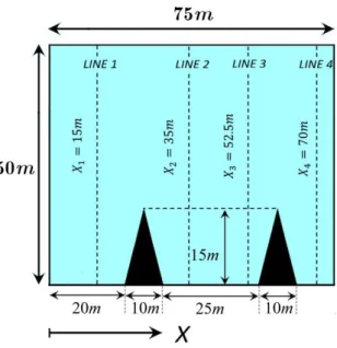
In order to compare the FDTD and TDWP methods, a simulation is set up as shown in fig. 8, containing two conducting triangles in free space. The ground plane is also assumed to be a perfect electrical conductor. The dimensions of the simulated space are shown in fig.8.

Fig 8. Dimensions of the simulated space and structures used in simulation. Four different columns at four different distances, where the field components should be stored in order to compute the propagation factors

The fields used in this simulation are Gaussian derivative functions of time with a central frequency of 50 MHz and a bandwidth of 100 MHz. The spatial distribution is a Gaussian derivative function of height as well. The center of the spatial distribution is taken to be 15 m high. The stimulation source is assumed to consist of a number of dipoles perpendicular to the ground. Therefore, the polarization is TM along the x direction. We would like to obtain the propagation factor as a function of height for four different distances, as shown in fig. 8. We compute the desired factors by two different procedures. In the first procedure, the simulation is performed for the whole space (using FDTD method) as shown in fig. 9 and the results are recorded.

(11)

Fig 9. Instantaneous images captured for comparing the FDTD and TDWP methods in the setup shown in fig.8

Propagation factor curves derived from these two methods are shown in fig.10. It can be seen that the two

curves do not match perfectly. The reason can be deduced by analyzing the images in fig. 9.

(12)

Brazilian Microwave and Optoelectronics Society-SBMO received 26 Jan 2018; for review 09 Feb 2018; accepted 16Aug 2018 Brazilian Society of Electromagnetism-SBMag © 2018 SBMO/SBMag ISSN 2179-1074 neither propagated back into the first window, nor absorbed by the PML located at the left boundary of the second window.Instead, the reflection is re-reflected into the second window.

The reason the reflected wave from the second triangle is not reflected back into the first window is obvious. As consequent computational spaces are discrete, i.e. not continuously connected as in the FDTD method, when the wave front passes through a window for which calculations are over, no field will be regenerated in the previous windows. It is apparent that should we apply the method we use to store fields yielded from previous window and regenerate the field in current window in reverse direction, the result would be a heavy computational burden as FDTD. The waves reflected from the second triangle are absorbed by the PML blocks located at the right and top borders of the window; however, they are reflected by the left border. The reason is that the first column in the window is regenerating fields from the last window during the whole duration of the simulation. In other words, these cells do not take part in the wave propagation that happens in the right to left direction and solely represent the values stored from the previous window. It may seem that when the reflected

wave from the second triangle reaches this column, the column’s cells are not regenerating any field.

(13)

Fig 10. Comparison between propagation losses for lines , , , and , obtained from FDTD and TWDP

B. Limiting field regeneration in the first column of the second window cells

(14)

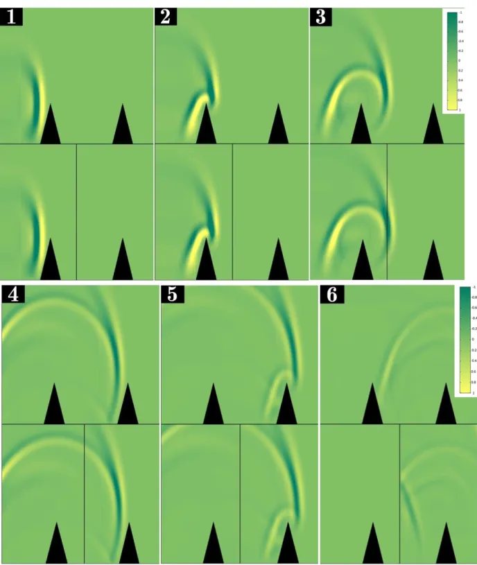
Fig11. Comparison of the instantaneous images taken, with field regeneration in the first column of the second window cells a) not limited b) limited.

Frames 1 to 6 demonstrate snapshots taken from the 608th through 928th time steps of the simulation, with 64 time steps between each two consecutive frames.

If the propagation factor computed for lines and using the modified simulation method is compared with FDTD, it can be observed that the modified TDWP method provides results closer to

a - 1

a - 2

a - 3

a - 5

a - 4

a - 6

b - 1

b - 2

_{b - 3}

(15)

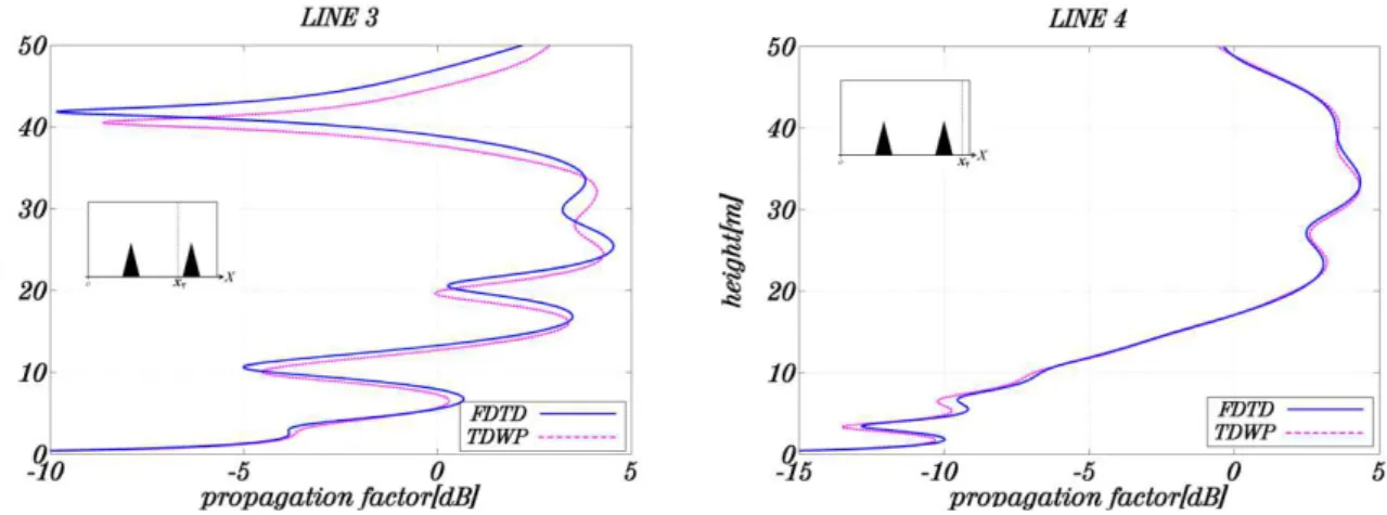
Brazilian Microwave and Optoelectronics Society-SBMO received 26 Jan 2018; for review 09 Feb 2018; accepted 16Aug 2018 Brazilian Society of Electromagnetism-SBMag © 2018 SBMO/SBMag ISSN 2179-1074 the results derived from FDTD [5]. Fig 12, shows the comparison between the propagation loss results of two method, Optimized TDWP and FDTD, in Lines 3 and 4.

Fig 12. Comparison of the propagation loss calculated using FDTD and modified TWDP for lines and , with field regeneration duration limited in the second window.

As it can be sometimes impossible to predict the time when wave reflection from the terrain reaches the end of the previous window, field regeneration duration cannot be limited in general. This problem can be solved by applying the substitution , where can be any field component , , or , and represents the stored value of the component from the last stage. It might seem that the aforementioned substitution causes new values to sum up with old values; but it must be borne in mind that field regeneration takes place when the field component values are being updated, so that every time a value is updated, it does not contain the previous value anymore.

C. Analysis of Improving Factors of Optimized TDWP Method

In following some relations are defined which can help us to make a suitable analysis regarding the efficiency of proposed Technics, in order to improve traditional TDWP method.

If we denote the propagation loss factor of Traditional and our Optimized TDWP method as

) (op TDW P

PF and PF_{TDW P}₍_re₎, respectively, the amount of generated Error in terms of y (axis) will be calculated for Traditional and Optimized methods as below, respectively. It should be emphasized that the one-window FDTD method is not applicable for long pathes. It is applied to this study just for a path of 100 m.

 

TDW Pre FDTD re

FDTD op

TDW P op

PF PF

y

PF PF

y

 

) (



(14)

(16)

 

_{ }

 

y

cf

re op





(15)

For investigating the improving factor of proposed method in one given line (like 0 yH , 

x



), we should first calculate the below Integrals for each line.

 











H re re H op op

dy

y

dy

y

0 0



(16)

The ratio of



_re to _op is defined as a Improving Factor for each vertical line x.

 

re op

x

CF





(17)

In similar way, for calculating the propagation loss factor along a horizontal line (like

0 

x



L

, 

y



) we will have :

(18)

 

TDW Pre FDTD re FDTD op TDW P op PF PF x PF PF x     ) ( ) (



The ratio of



_op

 

x to



_re

 

x

can be defined as improving factor for each length of x.

 

_{ }

 

x

cf

re op





(19)

For investigating the improving factor of proposed method in one given line (like 0 yH , 

y



), we should first calculate the below Integrals for each line.

 











L re re L op op

dx

x

dx

x

0 0



(20)

The ratio of _opto



_re is defined as a Improving Factor for each vertical line x.

 

re op

y

CF





(21)

At last, for attaining to a total improving factor in one window, relation 16 (or 20) should be employed over a given surface like



 

(17)

Brazilian Microwave and Optoelectronics Society-SBMO received 26 Jan 2018; for review 09 Feb 2018; accepted 16Aug 2018 Brazilian Society of Electromagnetism-SBMag © 2018 SBMO/SBMag ISSN 2179-1074 While this factor will be

CF



x



70 



0 .

05

for

x

_



70 m



Line

4 

. It shows that this technic make a better operation for

Line

4

in comparison to

Line

3

.

V. CONCLUSION

In this paper, the TDWP method for wave propagation simulation and propagation loss computation was introduced. The benefits of this method in comparison to the FDTD method where discussed, and by comparing these two methods for a terrain with two simulation windows, the shortcomings of TDWP methods where demonstrated. After that, by proposing the approach of limiting field regeneration for first column cells of each window, the matching between the propagation factors curves derived from the two methods was ameliorated. The TDWP method enables wave propagation simulation with personal computers; but provides better results for plain surfaces rather than for terrains. Such as the simulation of wave propagation for islands located near coasts where surface impedance changes as a function of distance from the source. In order to achieve more accurate results for surfaces with terrains, modifications should be made, as discussed above.

REFERENCES

[1] Sevgi, L., Ponsford, A., Chan, H.C., "An Integrated Maritime Surveillance System Based on High-Frequency Surface-Wave Radars, Part1: Theoretical Background and Numerical Simulations", IEEE Magazine, Vol. 43, No. 4, Agust, 2001.

[2] Akleman, F., Ozyalcin, M.O., Sevgi, L.,"Novel Time Domain Radiowave Propagators for Wireless Communication Systems", Turk. J. Elec. Engin.(TUBITAK), Vol.10, No. 2, 2002.

[3] Sevgi, Levent. "Groundwave modeling and simulation strategies and path loss prediction virtual tools." IEEE Transactions on Antennas and Propagation Vol.55, No.6, 2007.

[4] Okamoto, Hideaki, Koshiro Kitao, and Shinichi Ichitsubo. "Outdoor-to-indoor propagation loss prediction in 800-MHz to 8-GHz band for an urban area." IEEE Transactions on vehicular Technology Vol.58, No.3, 2009.

[5] Thomas, Timothy A., et al. "A prediction study of path loss models from 2-73.5 GHz in an urban-macro environment." Vehicular Technology Conference (VTC Spring), 2016 IEEE 83rd. IEEE, 2016.

[6] Sendra, Sandra, et al. "Underwater wireless communications in freshwater at 2.4 GHz." IEEE Communications Letters Vol.17, No.9, 2013.

[7] Li, Yujia, and J-M. Jin. "A vector dual-primal finite element tearing and interconnecting method for solving 3-D large-scale electromagnetic problems." IEEE Transactions on Antennas and Propagation Vol.54, No.10, 2006.

[8] Taflove, Allen, and Susan C. Hagness. Computational electrodynamics: the finite-difference time-domain method. Artech house, 2005.

[9] Peng, Zhen, Kheng-Hwee Lim, and Jin-Fa Lee. "Nonconformal domain decomposition methods for solving large multiscale electromagnetic scattering problems." Proceedings of the IEEE Vol.101, No.2, 2013.

[10] Gibson, Walton C. The method of moments in electromagnetics. CRC press, 2014.

[11] Berenger, J. p., "Perfectly Matched layer for the FDTD Solution of Wave-Structure Interaction Problem", IEEE Transactions on Antennas and Propagation, Vol. 44, No. 1, January 1996.