An intelligent support system for automatic detection of cerebral vascular accidents from brain CT images

Comput Methods Programs Biomed •

• •

. 2017 Jul;146:109-123.

doi: 10.1016/j.cmpb.2017.05.005. Epub 2017 May 20.

I.

An Intelligent Support System for

Automatic Detection of Cerebral

Vascular Accidents From Brain CT

Images

Elmira Hajimani1, M G Ruano2, A E Ruano3

Affiliations expand

• PMID: 28688480

An Intelligent Support System for Automatic Detection of Cerebral Vascular

Accidents from Brain CT Images

Elmira Hajimania,*, M.G. Ruanob, A. E. Ruanoc

a _{Faculty of Science and Technology, University of Algarve, Faro, Portugal, (e-mail:}

ehajimani@csi.fct.ualg.pt).

b _{Faculty of Science and Technology, University of Algarve, Faro, Portugal and CISUC,}

University of Coimbra, Portugal (e-mail: mruano@ualg.pt)

c _{Faculty of Science and Technology, University of Algarve, Faro, Portugal and IDMEC,}

Instituto Superior Técnico, University of Lisbon, Portugal, (e-mail: aruano@ualg.pt )

*_{Corresponding author. Tel: (+351) 915 918 528. Postal address: Lab. 2.75, FCT, Universidade}

do Algarve, Campus Gambelas, 8005-139 Faro, Portugal.

Abstract

Objective: This paper presents a Radial Basis Functions Neural Network (RBFNN) based detection system, for automatic identification of Cerebral Vascular Accidents (CVA) through analysis of Computed Tomographic (CT) images.

Methods: For the design of a neural network classifier, a Multi Objective Genetic Algorithm (MOGA) framework is used to determine the architecture of the classifier, its corresponding parameters and input features by maximizing the classification precision, while ensuring generalization.

This approach considers a large number of input features, comprising first and second order pixel intensity statistics, as well as symmetry/asymmetry information with respect to the ideal mid-sagittal line.

Results: Values of specificity of 98% and sensitivity of 98% were obtained, at pixel level, by an ensemble of non-dominated models generated by MOGA, in a set of 150 CT slices (1,867,602 pixels), marked by a NeuroRadiologist. This approach also compares favorably at a lesion level with three other published solutions, in terms of specificity (86% compared with 84%), degree of coincidence of marked lesions (89% compared with 77%) and classification accuracy rate (96% compared with 88%).

Keywords: Neural Networks; Symmetry features; Multi-Objective Genetic Algorithm; Intelligent

1. Introduction

Cerebral Vascular Accident (CVA), also called stroke, is caused by the interruption of blood supply to the brain, mainly due to a blood vessel blockage (i.e., ischemic), or by a haemorrhagic event. The cut-off of oxygen and nutrients supplies causes brain tissue irreversible damages, if not detected during the first 2-3 hours. Stroke accounted for approximately1 of every 19 deaths in the United States in 2009, according to [1]. Computed Tomography (CT) is the most commonly used CVA imaging diagnosis modality, available at almost all emergency units. When CVA is timely diagnosed, morbidity and mortality are minimised [2].

The increasing occurrence of CVAs in developed and developing countries, together with the insufficient number of Neuroradiologists and the lack of full-time expert Radiologists in some institutions, exacerbated by the fact that each exam is constituted by several images requiring an accurate analysis, leads to delays on the production of the clinical final report and subsequent clinical treatment, compromising the CVA’s recovery prognosis. In addition, at early stages of CVA, changes in the tomographic images may not be perceived by the human eye due to the inconspicuousness of the lesions.

For these reasoning, the existence of an automated system would be of paramount importance to detect subtle alterations, motivating the authors to create a computational intelligent application capable of assisting the Neuroradiologist in the analysis of CT scan images. The proposed application envisage enabling a preliminary trigger of a pathologic occurrence and a better performance of the CVA green line.

In this paper, a Radial Basis Functions Neural Network (RBFNN) based system is proposed for automatic detection of CVAs from brain CT images. The majority of the existing methods for designing the neural network classifier do not use an approach that determines the model structure that best fits the application at their hand, while simultaneously selecting the best input features. Moreover, their design typically does not consider multiple conflicting objectives such as minimization of the number of False Detections (FD) in the training dataset while achieving a desired level of model generalization, or, maximising the classification precision while reducing the model complexity. For this purpose, an hybrid of a multi-objective evolutionary technique is used as a design framework for features and topology selection, and, state-of-the-art derivative based algorithms are used for neural network parameter estimation, taking into account multiple objectives, as well as their corresponding restrictions and priorities [2, 3].

Moreover, to the best of our knowledge, none of existing classifiers consider the asymmetry caused by lesions in the intracranial area. In the proposed approach, a group of symmetry features that were proposed in [4], is used along with other statistical features, as inputs to the designed classifier.

The rest of the paper is organized as follows: Section 2 provides an overview of existing lesion segmentation strategies. The data acquisition process is explained in section 3. Section 4 describes

the features that are used in this study. Section 5 explains how the Multi Objective Genetic Algorithm (MOGA) is used to automatically design the RBFNN classifier. Experimental formulations and results are given in section 6. Section 7 discusses the results obtained in comparison with other published approaches. Conclusions are drawn in section 8.

2. Related works

Based on [5], a review of different lesion segmentation approaches, one can divide lesion segmentation strategies into two subgroups: supervised and unsupervised strategies.

Supervised approaches are those that use some kind of a priori information to perform the lesion segmentation. The group of supervised strategies can be further subdivided into two sub-groups: a) In the first subgroup, all approaches use atlas information, therefore requiring the application of a registration process to the analyzed image to perform the segmentation.

As an example, the authors in [6] used a combination of two techniques for brain lesion detection from CT perfusion maps: finding asymmetries among the two hemispheres and then comparing the captured images to a brain atlas anatomy. For generating the asymmetry map, first the symmetry axis is approximated as the straight line that minimizes the least square error between all centers of masses’ coordinates, and then the intensity values of the corresponding pixels on the left and right side of the image are compared. Those pixels with a significant difference are considered as potential lesions. To perform a detailed description of lesions a second step is required, where position image registration of the brain template is made. The goal of the registration algorithm is to maximize the similarity between the template image and the newly acquired image.

The work done in [7] can also be considered in this subgroup. This study presents an automated template-guided algorithm for the segmentation of ventricular CerebroSpinal Fluid (CSF) from ischemic stroke CT images. In the proposed method, the authors use two ventricular templates, one extracted from a normal brain (VT1) and the other built from several pathological scans (VT2). VT1 is used for registration and VT2 to define the region of interest. In the registration process, they use the Fast Talairach Transformation [8], which takes care of the “tilting” angle. Automatic thresholding is applied on a slice-by-slice basis, to cater for the variability of CSF intensity values across the slices in the same scan. The distributions of the CSF, White Matter (WM) and Gray Matter are analyzed and only voxels in the CSF range and WM range are used in the calculation of the histogram, employed by Otsu’s automatic thresholding algorithm [9]. Finally, artifacts are removed with the help of VT2.

b) All approaches which perform an initial training step on features extracted from manually segmented images, annotated by Neuroradiologists, can be considered as another subgroup of supervised strategies [5]. In this subgroup, different classifiers, such as Artificial Neural Networks, k-Nearest Neighbors, AdaBoost, Bayesian classifiers or decision trees, alone or

combined, have been used to perform the segmentation. The work presented in this article can be considered in this category.

The method applied in [10] is also an example of this subgroup. Primarily the method uses morphology operations and wavelets based filtering for image denoising. Then asymmetric parts of the brain and their neighbors are extracted being considered as the region of interest for specifying relevant features (such as texture, contrast, homogeneity, etc). Finally, k-means clustering and Support Vector Machines (SVM) are used for classification and provide the contour of the brain tumor.

The work presented in [11] uses a wavelet based statistical method for classifying brain tissues into normal, benign and malignant tumours. The authors first obtain the second level discrete wavelet transform of each CT slice. The Gray Level Co-occurrence Matrix (GLCM) is then calculated over the low frequency part of the transformed image. Finally, features are calculated from the GLCM matrix. Genetic algorithms and principle component analysis are employed for feature selection and SVM for classification.

In [12] a computer tomography (CT) brain image analysis system is proposed, with four phases: enhancement, segmentation, feature extraction and classification. The enhancement phase reduces the noise using an edge-based selective median filter (ESMF); the segmentation phase extracts the suspicious region applying a modified version of a genetic algorithm; the feature extraction phase extracts the textural features from the segmented regions and the last phase classifies the image. To diagnose and classify the image, the authors used a RBFNN classifier.

Regarding unsupervised strategies, where no prior knowledge is used, two different sub-groups can also be identified:

• A sub-group of methods that segment the brain tissue to allow lesion segmentation. These approaches usually detect lesions as outliers on each tissue, rather than adding a new class to the classification problem. The works presented in [13] and [14] follow this strategy.

• A sub-group that uses only lesion properties for segmentation. These methods directly segment the lesions according to their properties, without providing tissue segmentation. The works described in [15, 16] belong to this category.

3. Data acquisition

A database of existing CT images was used in this prospective study. All images were obtained from the same Siemens equipment. Each exam, where no contrast was applied, was composed by two ranges, one to study the posterior fosse and the other covering the remaining of the brain (5/5 mm and 10/10 mm, respectively).

In order to collect the opinion of Neuroradiologists about pathologic areas within brain CT images in an accurate and convenient way, a web-based tool was developed [17]. Using this tool, the

existing database of CT images was used for Neuroradiologists to analyze and mark the images either as normal or abnormal. For the abnormal ones, the doctor was asked to designate the lesion type and to manually trace the contours of abnormal region(s) on each CT’s slice image. Figure 1 shows the activity diagram of the Neuroradiologist in the developed tool.

The administrator of the developed web-based tool can then download a text file in which the coordinates of each marked pixel (i.e., a lesion) are specified. These pixels are considered as abnormal data samples. The resolution of each CT slice is 512 × 512 pixels and the intensity value of each pixel is an integer in the range [0 255], 0 being completely black and 255 completely white. Within a CT slice, all the intracranial pixels which are not marked as lesions will be considered as normal data samples.

Our collaborating Neuroradialogist registered his opinion for 7 patients (150 CT slices). 24 out of the 150 CT slices had lesions within their intracranial area, corresponding to 64,786 abnormal pixels. All lesions were marked as ischemic stroke. To obtain the coordinates of all normal pixels, Algorithm 1 (described below) is used. It calls Algorithm 2 (described afterwards) for artifact removal on each image. Applying Algorithm 1, we obtained 1,802,816 normal pixels. As a result, we have a total of 1,867,602 normal and abnormal pixels to work with.

Figure1. Activity diagram of the Neuroradiologist in the data acquisition tool

Algorithm 1 Obtaining the coordinate of normal pixels

Input: text file, say T, where the coordinate of abnormal pixels and the path from which the

image can be retrieved are saved.

1. Let 𝐸𝑥𝑎𝑚𝑠 be a structure that is constructed from text file T. 𝐸𝑥𝑎𝑚𝑠(𝑖) contains the information of each CT exam.

2. For 𝑖 = 1 to 𝑙𝑒𝑛𝑔𝑡ℎ(𝐸𝑥𝑎𝑚𝑠)

2.1. Pass 𝐸𝑥𝑎𝑚𝑠(𝑖) through Algorithm 2, to remove the skull and other artifacts. 2.2. For each image in 𝐸𝑥𝑎𝑚𝑠(𝑖)

2.2.1. Let 𝑋, 𝑌 be two vectors containing the location of abnormal pixels 2.2.2. Let 𝑃(𝑎, 𝑏) be the intensity of the pixel located in (𝑎, 𝑏)

2.2.3. If 𝑃(𝑎, 𝑏) ≠ 0 and 𝑎 ∉ 𝑋 and 𝑏 ∉ 𝑌

2.2.3.1. Insert (𝑎, 𝑏) and 𝑝𝑎𝑡ℎ(𝑖𝑚𝑎𝑔𝑒) as a row in a text file O. End if

End for End for

Output: text file O

Algorithm 2 Artifact removal algorithm in brain CT images [18]

Input: Brain CT images of one examination

1. Skull detection:

1.1. Remove pixels whose intensities are less than 250.

1.2. Use the Connected Component algorithm [19] to choose the largest component as the candidate skull.

1.3. Remove the small holes within the candidate skull, by inverting the matrix of candidate skull and applying the Connected Component algorithm for the second time. Those connected components whose area are less than 200 pixels are considered as holes and will be filled using the bone intensity value

2. Removing CT slices with either unclosed skulls or skull containing too many separate regions: Having completed step 1.3, we have already all connected components at hand. As a result, we can count the number of big holes (e.g., areas more than 200 pixels wide). If this number is equal to 2, it will be considered as closed skull; otherwise the slice will be removed from the desired set.

3. Intracranial area detection: All CT images that successfully passed step 2 contain only two black regions separated by the skull. To detect which black area is related to the intracranial part, the mass centre of the skull is calculated, the region containing the mass centre being considered as intracranial area.

Output: Intracranial part of a subset of input CT images.

4. Feature space

Having a set of pixel coordinates whose labels (normal or abnormal) are already determined by expert, we are now able to produce our dataset by extracting the corresponding features from the images. Each CT image is represented as a matrix 𝐼 with 𝑀 rows and 𝑁 columns where 𝐼(𝑚, 𝑛) stands for the intensity of pixel in row 𝑚 and column 𝑛. Three groups of features are used to construct the feature space: first order statistics, second order statistics and symmetry features. Table I describes the 51 features considered. First order statistics estimate properties of individual pixel values (e.g. 𝑓1 to 𝑓16 and 𝑓37 to 𝑓41), ignoring the spatial interaction between the image pixels. Second order features estimate properties of two pixel values occurring at specific locations relative to each other by constructing a Gray Level Co-occurrence Matrix. To extract some of the first and second order statistical features, a window 𝑤 of size 31*31 [20, 21] centered at the pixel (𝑥, 𝑦) is employed.

The variance of pixel intensities within a window 𝑤 is denoted by 𝑣𝑎𝑟_𝑤. Given 𝑤 centred at point (𝑥, 𝑦) , L_h is a row vector with the intensities of the 31 pixels taken from the horizontal line centered at (𝑥, 𝑦) and L_v is a column vector with the intensities of the 31 pixels taken from the

vertical line centered at (𝑥, 𝑦). For calculating features 𝑓15, 𝑓16 and 𝑓38 to 𝑓41, 𝐿 = 8 gray levels of the histogram of pixel intensities within window 𝑤 are calculated. Each bin of histogram is represented by 𝐻𝑙.

A GLCM matrix is a two-dimensional matrix 𝐶 where both the rows and the columns represent a set of possible image values G (e.g. gray tones). The value of 𝐶(𝑖 , 𝑗) indicates how many times the value 𝑖 co-occurs with value 𝑗 in some designated spatial relationship. The spatial relationship is usually defined by a distance 𝑑 and a direction 𝜃. In this study, to calculate the 8 gray level GLCM of 𝑤, the displacement parameters considered were 𝑑 = 1 and 𝜃 = 0,45,90,135. As a result, 4 GLCM matrices are derived, each one belonging to one specific 𝜃 and then the average is computed in order to obtain a direction invariant GLCM matrix.

In the formulas used in Table I, the mean value of matrix 𝐶 is represented by 𝜇 and the mean and standard deviation for the rows and columns of 𝐶 are defined in (1) and (2) respectively.

𝜇𝑥 = ∑ 𝑖. 𝐶(𝑖, 𝑗) 𝑖,𝑗 , 𝜇𝑦 = ∑ 𝑗. 𝐶(𝑖, 𝑗)𝑖,𝑗 (1)

𝜎𝑥 = ∑ (𝑖 − 𝜇𝑖,𝑗 𝑥)2. 𝐶(𝑖, 𝑗) , 𝜎𝑦 = ∑ (𝑗 − 𝜇𝑦) 2

. 𝐶(𝑖, 𝑗)

𝑖,𝑗 (2)

Moreover, 𝐶_𝑥(𝑖) is the ith _{entry in the marginal-probability matrix obtained by summing the rows}

of 𝐶(𝑖, 𝑗) and 𝐶_𝑦(𝑖) is obtained by summing the columns of 𝐶(𝑖, 𝑗).

Given the ideal mid-sagittal line, symmetry features aim to compare one side of the brain to the other side and discover if there are any suspicious differences. To detect the ideal midline and to rotate tilted images to make the ideal midsagittal line perpendicular to the x-axis, the method summarized in Algorithm 3 is employed.

Algorithm 3 Ideal midline detection of the brain CT [18, 22]

Input: Brain CT images of one exam

1. Use Algorithm 2 to remove artifacts.

2. Since the concave shape of intracranial region will affect the accuracy of search for finding ideal midline, CT slices with high amount of concavity are found and excluded:

2.1. For each CT slice

2.1.1. Extract the contour of intracranial region. 2.1.2. 𝐶𝑜𝑛𝑐𝑎𝑣𝑖𝑡𝑦 = 0

2.1.3. For ∅ = 0 to 180

2.1.3.1. Rotate contour by ∅ degree. 2.1.3.2. 𝐶𝑜𝑛𝑐𝑎𝑣𝑖𝑡𝑦∅= 0

2.1.3.3. For 𝑖 = 1 to 𝑛𝑢𝑚𝑏𝑒𝑟 𝑜𝑓 𝑟𝑜𝑤𝑠

2.1.3.3.1. Scan the pixels of the contour in row 𝑖 and define the Far Left (𝐹𝐿𝑖) and Far Right (𝐹𝑅𝑖) junctions.

2.1.3.3.2. Let 𝐶𝑖 be the number of pixels in row 𝑖 which reside between 𝐹𝐿𝑖 and 𝐹𝑅𝑖 and that are not located inside the intracranial region.

2.1.3.3.3. 𝐶𝑜𝑛𝑐𝑎𝑣𝑖𝑡𝑦∅= 𝐶𝑜𝑛𝑐𝑎𝑣𝑖𝑡𝑦∅+ 𝐶𝑖 End for

2.1.3.4. 𝐶𝑜𝑛𝑐𝑎𝑣𝑖𝑡𝑦+= 𝐶𝑜𝑛𝑐𝑎𝑣𝑖𝑡𝑦∅ End for

End for

2.2. Sort CT slices based on their corresponding 𝐶𝑜𝑛𝑐𝑎𝑣𝑖𝑡𝑦 values and select the first 𝜆 slices with the least amount of concavity.

3. To find the line that maximizes the symmetry of the resulting halves, a rotation angle search around the mass centre of the skull is performed:

3.1. For each CT slice remaining from step 2:

3.1.1. Let 𝜃 be the maximum angle that a given CT image can be tilted. 3.1.2. Let 𝑆𝑗 be the symmetry cost at angle 𝑗

3.1.3. For 𝑗 = −𝜃 to 𝜃

3.1.3.1. Calculate 𝑆𝑗= ∑𝑛𝑖=1|𝑙𝑖− 𝑟𝑖| where 𝑛 is the number of rows in the current CT slice, 𝑙𝑖 and 𝑟𝑖 are the distances between the current approximate midline and the left and right side of the skull edge in row, respectively.

End for

3.1.4. Select rotation angle 𝑗 whose symmetry cost 𝑆𝑗 is minimum. End for

3.2. The final rotation degree for all CT slices is determined as the median value of rotation angles obtained for each CT slice.

4. Rotate all CT slices around their corresponding skull mass centre based on the rotation degree obtained in step 3.2

5. Line 𝑥 = 𝑥𝑚𝑎𝑠𝑠 𝑐𝑒𝑛𝑡𝑒𝑟(𝑖) is considered as the ideal midline of the brain CT image 𝑖.

Output: CT images are aligned and their corresponding ideal midlines determined.

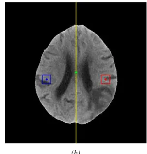
To extract symmetry features, a window 𝑤₁of size 𝑠 × 𝑠 centred at pixel (𝑥, 𝑦), marked by a clinical expert as normal or abnormal, and its contralateral part with respect to the midline, window 𝑤₂ centred at the pixel (𝑥′, 𝑦′), are considered (please see Figure 2-b).

(a) (b)

Figure 2. (a) Original brain CT image; (b) After skull removal and realignment, the ideal midline is drawn in yellow. The green point shows the mass centre (centroid) of the skull upon which the alignment rotation is performed. A window of size 31x31 is considered around the pixel located

at (365,279) and shown in red; its contralateral part with respect to the midline is shown in blue [4].

Having identified 𝑤₁ and 𝑤₂, we can then specify how similar these two regions are by calculating the Pearson Correlation Coefficient (PCC), as stated in (3). The 𝐿1 norm and squared 𝐿2 norms

are also two dissimilarity measures that can be obtained using (4) and (5), respectively. Comparing the intensity value of the pixel that is marked by the expert, and its corresponding pixel in the contralateral part, another symmetry feature defined in (6) can be obtained.

𝑃𝐶𝐶 =1 𝑛∑ ∑ ( 𝐼_𝑤1𝑖,𝑗−𝜇_𝑤1 𝜎_𝑤1 ) ( 𝐼_𝑤2𝑖,𝑗−𝜇_𝑤2 𝜎_𝑤2 ) 𝑠 𝑗=1 𝑠 𝑖=1 (3) 𝐿1 = ∑ ∑ |𝐼𝑤1 𝑖,𝑗 − 𝐼_𝑤𝑖,𝑗₂| 𝑠 𝑗=1 𝑠 𝑖=1 (4) 𝐿2_{2 = ∑ ∑ (𝐼} 𝑤1 𝑖,𝑗 − 𝐼_𝑤𝑖,𝑗₂)2 𝑠 𝑗=1 𝑠 𝑖=1 (5) 𝑑𝑖𝑓𝑓 = 𝐼_𝑤𝑥,𝑦₁ − 𝐼_𝑤𝑥₂′,𝑦′ (6) In the previous equations, 𝐼𝑖,𝑗 is the intensity value of pixel located at (𝑖, 𝑗) within the corresponding window; 𝜇_𝑤1, 𝜎𝑤1 𝜇𝑤2, and 𝜎𝑤2 are the mean and standard deviation of the

intensity values within window 𝑤₁ and its contralateral part, window 𝑤₂ , respectively. In Table I, 𝑓42 to 𝑓51 are symmetry features for three different window sizes ({11,21,31} ).

In Table I, features 𝑓1 to 𝑓13 are taken from [21]; 𝑓13 to 𝑓16 are used in [23]; 𝑓17 to 𝑓23 and 𝑓25 to 𝑓34 are from [24]; 𝑓24 is a built-in MATLAB function; 𝑓35 and 𝑓36 are used in [25]; 𝑓38 to 𝑓41 are obtained from [20] and 𝑓42 to 𝑓51 were proposed in [4].

Table I. Features considered

Description 𝑓1 𝐼(𝑥, 𝑦) 𝑓2 min 𝑚,𝑛 ∈ 𝑤𝐼(𝑚, 𝑛) 𝑓3 average 𝑚,𝑛 ∈ 𝑤 𝐼(𝑚, 𝑛) 𝑓4 max 𝑚,𝑛 ∈ 𝑤𝐼(𝑚, 𝑛) 𝑓5 median 𝑚,𝑛 ∈ 𝑤 𝐼(𝑚, 𝑛) 𝑓6 std𝑤=( 1 𝑤𝑖𝑑𝑡ℎ(𝑤)×ℎ𝑒𝑖𝑔ℎ𝑡(𝑤)−1× ∑ ∑ (𝐼(𝑚, 𝑛) − 𝑓3) 2 𝑦+(𝑤𝑖𝑑𝑡ℎ(𝑤)−1)₂ 𝑛=𝑦−(𝑤𝑖𝑑𝑡ℎ(𝑤)−1)₂ 𝑥+(ℎ𝑒𝑖𝑔ℎ𝑡(𝑤)−1)₂ 𝑚=𝑥−(ℎ𝑒𝑖𝑔ℎ𝑡(𝑤)−1)₂ ) 1/2 𝑓7 average 1≤𝑚≤𝑀, 1≤𝑛≤𝑁 𝐼(𝑚, 𝑛) 𝑓8 average 𝑚,𝑛 ∈ 𝑤 𝐼(𝑚, 𝑛) − average 1≤𝑚≤𝑀, 1≤𝑛≤𝑁 𝐼(𝑚, 𝑛) 𝑓9 𝐼(𝑥, 𝑦) − average 1≤𝑚≤𝑀, 1≤𝑛≤𝑁 𝐼(𝑚, 𝑛) 𝑓10 Plh = ∑ |Lh(x, n + 1) − Lh(x, n)| 𝑦+(𝑤𝑖𝑑𝑡ℎ(𝑤)−1) 2 𝑛=𝑦−(𝑤𝑖𝑑𝑡ℎ(𝑤)−1)₂ 𝑓11 plv = ∑𝑥+ |L_v(m + 1, y) − L_v(m, y)| (ℎ𝑒𝑖𝑔ℎ𝑡(𝑤)−1) 2 𝑚=𝑥−(ℎ𝑒𝑖𝑔ℎ𝑡(𝑤)−1) 2 𝑓12 cxm =𝑥/512 𝑓13 Skewness= 1 𝑣𝑎𝑟𝑤3∑ ∑ (𝐼(𝑚, 𝑛) − 𝑓3) 3 𝑦+(𝑤𝑖𝑑𝑡ℎ(𝑤)−1) 2 𝑛=𝑦−(𝑤𝑖𝑑𝑡ℎ(𝑤)−1)₂ 𝑥+(ℎ𝑒𝑖𝑔ℎ𝑡(𝑤)−1) 2 𝑚=𝑥−(ℎ𝑒𝑖𝑔ℎ𝑡(𝑤)−1)₂ 𝑓14 Kurtosis= 1 𝑣𝑎𝑟𝑤4 ∑ ∑𝑦+ (𝐼(𝑚, 𝑛) − 𝑓3)4 (𝑤𝑖𝑑𝑡ℎ(𝑤)−1) 2 𝑛=𝑦−(𝑤𝑖𝑑𝑡ℎ(𝑤)−1) 2 𝑥+(ℎ𝑒𝑖𝑔ℎ𝑡(𝑤)−1)₂ 𝑚=𝑥−(ℎ𝑒𝑖𝑔ℎ𝑡(𝑤)−1) 2 𝑓15 _{Energy=∑ (} 𝐻𝑙 𝑤𝑖𝑑𝑡ℎ(𝑤)×ℎ𝑒𝑖𝑔ℎ𝑡(𝑤)) 2 L l=1 𝑓16 _{Entropy=− ∑} 𝐻𝑙 𝑤𝑖𝑑𝑡ℎ(𝑤)×ℎ𝑒𝑖𝑔ℎ𝑡(𝑤)log2{ 𝐻𝑙 𝑤𝑖𝑑𝑡ℎ(𝑤)×ℎ𝑒𝑖𝑔ℎ𝑡(𝑤)} L l=1 𝑓17 Autocorrelation=∑𝑖,𝑗(𝑖𝑗)𝐶(𝑖, 𝑗) 𝑓18 _Correlation=∑ (𝑖𝑗)𝐶(𝑖,𝑗)𝑖,𝑗 −𝜇𝑥𝜇𝑦 𝜎𝑥𝜎𝑦 𝑓19 _{Cluster Prominence=∑ (𝑖 + 𝑗 − 𝜇} 𝑥− 𝜇𝑦) 4 𝐶(𝑖, 𝑗) 𝑖,𝑗 𝑓20 _{Cluster shade=∑ (𝑖 + 𝑗 − 𝜇} 𝑥− 𝜇𝑦) 3 𝐶(𝑖, 𝑗) 𝑖,𝑗 𝑓21 Dissimilarity=∑ |𝑖 − 𝑗|. 𝐶(𝑖, 𝑗)𝑖,𝑗 𝑓22 GLCM Energy =∑𝑖,𝑗𝐶(𝑖, 𝑗)2 𝑓23 GLCM Entropy=− ∑ 𝐶(𝑖, 𝑗)log (𝐶(𝑖, 𝑗))𝑖,𝑗 𝑓24 _{Homogeneity= ∑} 𝐶(𝑖,𝑗) 1+|𝑖−𝑗| i,j

𝑓25 Homogeneity = ∑_i,jC(i, j) (1 + (i − j)⁄ 2)

𝑓26 Maximum probability=MAX

𝑖,𝑗 𝐶(𝑖, 𝑗)

𝑓27 Sum of squares =∑ (𝑖 − 𝜇)𝑖,𝑗 2𝐶(𝑖, 𝑗)

𝑓28 Sum average=∑2𝐺𝑖=2𝑖𝐶𝑥+𝑦(𝑖) where 𝐶𝑥+𝑦(𝑘) = ∑𝐺𝑖=1∑𝐺𝑗=1𝐶(𝑖, 𝑗)| 𝑖 + 𝑗 = 𝑘 , 𝑘 =

2,3, … ,2𝐺 𝑓29 Sum variance= ∑ (𝑖 − 𝑓30)2_𝐶 𝑥+𝑦(𝑖) 2𝐺 𝑖=2 where 𝐶𝑥+𝑦(𝑘) = ∑𝐺𝑖=1∑𝐺𝑗=1𝐶(𝑖, 𝑗)| 𝑖 + 𝑗 = 𝑘 , 𝑘 = 2,3, … ,2𝐺

𝑓30 Sum entropy=− ∑2𝐺_𝑖=2𝐶_𝑥+𝑦(𝑖)log (𝐶_𝑥+𝑦(𝑖)) where 𝐶_𝑥+𝑦(𝑘) = ∑𝐺_𝑖=1∑𝐺_𝑗=1𝐶(𝑖, 𝑗)| 𝑖 + 𝑗 = 𝑘 , 𝑘 = 2,3, … ,2𝐺

𝑓31 Difference variance= 𝑣𝑎𝑟𝑖𝑎𝑛𝑐𝑒 𝑜𝑓 𝐶_𝑥−𝑦 where 𝐶_𝑥−𝑦(𝑘) = ∑𝐺_𝑖=1∑𝐺_𝑗=1𝐶(𝑖, 𝑗)| 𝑖 − 𝑗 = 𝑘 , 𝑘 = 0,1, … , 𝐺 − 1 𝑓32 _{Difference entropy= − ∑ 𝐶} 𝑥−𝑦(𝑖) log (𝐶𝑥−𝑦(𝑖)) 𝐺−1 𝑖=0 where 𝐶𝑥−𝑦(𝑘) = ∑𝐺_𝑖=1∑𝐺_𝑗=1𝐶(𝑖, 𝑗)| 𝑖 − 𝑗 = 𝑘 , 𝑘 = 0,1, … , 𝐺 − 1 𝑓33 Information measure of correlation1= 𝑓23−𝐻𝑋𝑌1

max{𝐻𝑋 ,𝐻𝑌} where 𝐻𝑋 and 𝐻𝑌 are Entropies of 𝐶𝑥

and 𝐶_𝑦 and 𝐻𝑋𝑌1 = − ∑ 𝐶(𝑖, 𝑗)𝑙𝑜𝑔{𝐶_{𝑖,𝑗 𝑥}(𝑖)𝐶_𝑦(𝑗)}

𝑓34 _{Information measure of correlation2= (1 − 𝑒𝑥𝑝[−2.0(𝐻𝑋𝑌2 − 𝑓23)])}1⁄2 _where

𝐻𝑋𝑌2 = − ∑ 𝐶𝑥(𝑖)𝐶𝑦(𝑗)𝑙𝑜𝑔{𝐶𝑥(𝑖)𝐶𝑦(𝑗)} 𝑖,𝑗

𝑓35 _{Inverse difference normalized=∑} 𝐶(𝑖,𝑗) 1+|𝑖−𝑗| 𝐺⁄ 𝐺

𝑖,𝑗=1

𝑓36 _{Inverse difference moment normalized=∑} 𝐶(𝑖,𝑗) 1+(𝑖−𝑗)2_/𝐺2 𝐺 𝑖,𝑗=1 𝑓37 𝑉𝑎𝑟_𝑤= 1 𝑤𝑖𝑑𝑡ℎ(𝑤)×ℎ𝑒𝑖𝑔ℎ𝑡(𝑤)× ∑ ∑ (𝐼(𝑚, 𝑛) − 𝑓3) 2 𝑦+(𝑤𝑖𝑑𝑡ℎ(𝑤)−1)₂ 𝑛=𝑦−(𝑤𝑖𝑑𝑡ℎ(𝑤)−1) 2 𝑥+(ℎ𝑒𝑖𝑔ℎ𝑡(𝑤)−1)₂ 𝑚=𝑥−(ℎ𝑒𝑖𝑔ℎ𝑡(𝑤)−1) 2 𝑓38 (𝐻1+ 𝐻2) (𝑤𝑖𝑑𝑡ℎ( 𝑤))⁄ 2 𝑓39 (𝐻₃+ 𝐻₄) (𝑤𝑖𝑑𝑡ℎ( 𝑤))_⁄ 2 𝑓40 (𝐻₅+ 𝐻₆) (𝑤𝑖𝑑𝑡ℎ( 𝑤))_⁄ 2 𝑓41 (𝐻₇+ 𝐻₈) (𝑤𝑖𝑑𝑡ℎ( 𝑤))_⁄ 2 𝑓42 𝑃𝐶𝐶 , 𝑠 = 31 𝑓43 𝑑𝑖𝑓𝑓 𝑓44 𝐿1 , 𝑠 = 31 𝑓45 𝐿2₂ , 𝑠 = 31 𝑓46 𝑃𝐶𝐶 , 𝑠 = 21 𝑓47 𝐿₁ , 𝑠 = 21 𝑓48 𝐿2₂ , 𝑠 = 21 𝑓49 𝑃𝐶𝐶 , 𝑠 = 11 𝑓50 𝐿1 , 𝑠 = 11 𝑓51 𝐿2₂ , 𝑠 = 11

5. Neural Network design using the Multi Objective Genetic Algorithm framework

The identification of Neural Network inputs, topology and parameters from data is often done iteratively in an ad-hoc fashion, focusing mainly on parameters identification. This is because the number of possibilities for the selection of the model structure (inputs and topology) are usually very large. Moreover, typically the design criterion is a single measure of the error obtained by the model, such as the mean-square error or the root-mean-square error, while typically the aim is to obtain a satisfactory performance (determined by typically more than one criterion) with small networks, i.e., the design problem should be formulated as a multiple-objective problem.

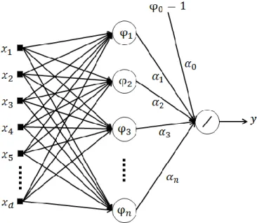
The model used for pixel classification is a Radial Basis Function Neural Network (RBFNN).

Figure 3. Topology of a RBFNN

The topology of a RBFNN is presented in Figure 3. The second layer units, known as neurons, are nonlinear functions of their vector inputs, given by,

𝜑𝑖(𝒙, 𝒄𝑖, 𝜎𝑖) = 𝑒

−‖𝒙−𝒄𝑖‖2

2𝜎_𝑖2 _{, 𝜑}

0 = 1, (7)

where ‖ ‖ denotes the Euclidean norm, and ci and 𝜎𝑖 are, respectively, the location of the Gaussian

function in the input space (denoted as centers) and its spread. The RBFNN output is given by:

𝑦(𝒙, 𝜶, 𝑪, 𝝈) = ∑ 𝛼_𝑖𝜑_𝑖(𝒙, 𝒄𝑖, 𝜎𝑖) = 𝝋(𝒙, 𝑪, 𝝈) 𝑛

𝑖=0

𝜶, (8)

As in this application the RBFNNs are used as classifiers, the output y is passed through a threshold function, in such a way that if y>0, the pixel is classified as abnormal, and normal otherwise. In order to identify the best possible Radial Basis Functions neural network structure and parameters, this work uses a Multi-Objective Genetic Algorithm (MOGA) design framework, described in, for instance, [2, 26]. This method also allows us to handle multiple, possibly conflicting objectives. MOGA finds a non-dominated set of individuals through 𝑛 number of generations and then selects preferable individuals from the non-dominated set. A solution is called non-dominated if none of the objectives can be improved in value without sacrificing some of the other objective values [27].

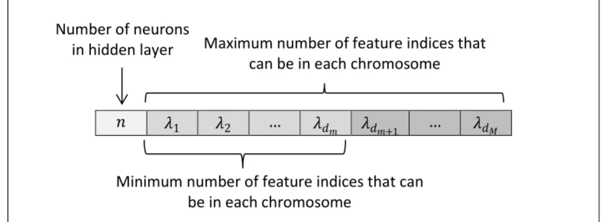
In order to be able to use the MOGA approach for finding the best possible model structure and its corresponding parameters, each possible structure for the NN needs to be formulated as a chromosome. To do that, the number of neurons in hidden layer is considered as the first component of the chromosome and the remaining components are the indices of features to be selected from a feature space. Figure 4 shows the topology of the chromosome. The algorithm starts its work by producing a pre-defined number of individuals as the first generation. The method then needs a mechanism to compare the individuals and select the best ones with respect to pre-defined objectives. The objectives, for the case at hand, can be selected from the set 𝑜𝑏𝑗 as described in (9).

𝑜𝑏𝑗 = {𝐹𝑁_𝑠 , 𝐹𝑃_𝑠 , 𝑀𝐶 | 𝑠 = {𝑇𝐸, 𝑇𝑅}} (9) where 𝐹𝑁_𝑠 is the number of False Negatives (i.e., those abnormal pixels that are wrongly classified as normal); 𝐹𝑃_𝑠 is the number of False Positives (i.e., those normal pixels that are wrongly classified as abnormal) and 𝑀𝐶 stands for the Model Complexity. 𝑇𝐸 and 𝑇𝑅 represent Test and Training sets respectively. The formula for calculating Model Complexity is given in (10).

Figure 4. The topology of the chromosome

𝑀𝐶 = (𝑁𝑢𝑚𝑏𝑒𝑟 𝑜𝑓 𝑖𝑛𝑝𝑢𝑡 𝑓𝑒𝑎𝑡𝑢𝑟𝑒𝑠 + 1) × 𝑁𝑢𝑚𝑏𝑒𝑟 𝑜𝑓 𝑛𝑒𝑢𝑟𝑜𝑛𝑠 𝑖𝑛 ℎ𝑖𝑑𝑑𝑒𝑛 𝑙𝑎𝑦𝑒𝑟 (10)

𝑛 𝜆1 𝜆2 … 𝜆𝑑𝑚 𝜆𝑑𝑚+1 … 𝜆𝑑𝑀

Minimum number of feature indices that can be in each chromosome

Number of neurons

in hidden layer Maximum number of feature indices that can be in each chromosome

For evaluating the individuals in one generation, each NN model is trained with the provided training dataset (i.e., using the features whose indices are depicted in chromosome). The Levenberg-Marquardt (LM) algorithm [28, 29], with a formulation that exploits the linear-nonlinear separability of the NN parameters [30, 31] is employed for training due to its higher accuracy and convergence rate. Training is terminated if an user-specified number of iterations is reached, or the performance on a test set reaches a minimum (a procedure known as early-stopping [32]).

Since the result of gradient-based methods, such as LM, depends on the model initial parameters’ values, for each individual in the current generation, the training procedure is repeated α times. Within these, the best result is picked up for determining the parameters of the individual (i.e., the centres, spreads and weights in RBFNNs). In MOGA, there are 𝑑 + 2 different ways for identifying which training trial is the best one, considering 𝑑 as the number of the objectives. The first strategy is to select the training trial which has minimized all objectives better than the others. In other words, if we consider a 𝑑 dimensional space, the one whose Euclidean distance from the origin is the smallest, will be considered as the best. The green arrow in Figure 5 indicates this situation for 𝑑 = 2. In the second strategy, the average of the objective values for all training trials is calculated and then the trial whose value is the closest to this average will be selected as the best one (i.e., the red arrow in Figure 5).

The other 𝑑 strategies are to select the training trial which minimized the 𝑖𝑡ℎ objective (𝑖 = 1,2, ⋯ , 𝑑) better than the other trials. As an example, the yellow and blue arrows in Figure 5 are the training trials which minimized objective1 and objective 2, respectively.

Having trained each individual, we are now able to assign a fitness value which reflects the individual’s quality. MOGA uses a Pareto-based fitness assignment approach, which was first proposed by Goldberg and then modified by Fonseca and Fleming [33]. In this method, the individuals are ranked according to the number of individuals by which they are dominated. For example, if an individual is non-dominated, its corresponding rank is 0 and if an individual is dominated by three other individuals, its corresponding rank will be 3. Figure 6 visualizes the Pareto ranking notion.

Figure 6. Pareto ranking [26, 34]

If there exists any preference such as assigning different priorities to each objective or defining a desired level of performance for each objective (i.e., restrictions), the ranking technique is slightly modified to take the restrictions and priorities into account. Suppose that 𝑐₁ and 𝑐₂ are the corresponding restrictions of objectives 1 and 2. In the case that both objectives have the same priorities, the individuals who satisfied the restrictions are assigned a rank equal to the number of individuals by which they are dominated. The individuals which do not meet the restrictions are penalized by assigning a higher rank. Figure 7 illustrates this situation.

0 0 0 0 2 1 1 3 5 Objective 1 Objecti ve 2

Figure 7. Pareto ranking in the case that both objectives have equal priorities. Both objectives should meet the defined restrictions [27, 33].

Figure 8 illustrates a situation in which objective 2 has a higher priority than objective 1. In this case, individuals which do not meet restriction 𝑐₂ are the worst, independently of their performance according to objective 1. Once 𝑐2 is met, individuals are ranked based on how well

they optimized objective 1 [27, 33].

0 0 5 5 5 1 1 3 5 Objective 1 Objecti ve 2 𝑐2 𝑐₁

Figure 8. Pareto ranking in the case that objective 2 has higher priority than objective 1. Both objectives should meet the defined restrictions [27, 33].

Having ranked the individuals, MOGA assigns a fitness value to each individual based on its corresponding rank. To do that, the individuals are sorted based on the ranks and the fitness is assigned by interpolating from the best individual (i.e., rank=0) to the worst according to a linear or exponential function. Finally, a single value of fitness is calculated for the individuals with the same rank by the means of averaging. Assigning the average value to those with the same rank will guarantee the same probability of being selected as the parent of next generation [33-35]. The mating procedure uses the fitness values to generate a new population, ensuring that the individuals with higher fitness have a larger probability of breeding. To generate a new population, a small percentage of random immigrant from the previous generation is also introduced into the population, which makes the genetic algorithm more likely to recover information lost through selection and thus, from genetic drift [33]. The pairs selected for mating exchange part of their chromosome (i.e., based on the given probability crossover rate), to produce two offsprings for each pair, in the recombination phase. Parent recombination is done in a way that the offspring respect the maximum model length. The resulting offspring may be longer, shorter or equally sized as their parents. Once the new population is generated after recombination, mutation is applied to randomly selected individuals. The mutation operator is implemented by three basic operations: substitution, deletion and addition of one element. The number of neurons is mutated, with a given probability, by adding or subtracting one neuron to the model, verifying boundary conditions such that no neural network can have fewer or more neurons than pre-specified values. Each model

0 2 5 8 7 1 3 4 6 Objective 1 Objecti ve 2 𝑐2 𝑐₁

input term in the chromosome is tested and, with a given probability, is either replaced by a new term not in the model, or deleted. Finally, a new term may be appended to the chromosome. In each MOGA iteration, as shown in Figure 9, the non-dominated set is updated based on the individuals in current generation. It is expected that, after a sufficient number of generations, the population has evolved to achieve a non-dominated set which is not going to be altered; in this stage, the user must select the best model, among the final non-dominated set.

Figure 9. The update of the non-dominated set on arrival of new points. The gray area denotes all generated models up to the current generation.

6. Experimental results

6.1. Constructing the input dataset for MOGA

Using the MOGA approach, the system must train a considerable amount of RBFNN models to be able to construct the final non-dominated set (please recall that the training process is done 𝜶=10 times for each chromosome). As a result, in practice, some constraints should be imposed on the size of the datasets that will be provided to MOGA, otherwise the process would not be finished in a reasonable time. As mentioned in section 3, we have 1,867,602 pixels (hereby called as 𝑩𝑰𝑮_𝑫𝑺) whose status (i.e., normal or abnormal) is already determined by the Neuroradiologist.

Among these pixels 1,802,816 are normal (96.53% of the data samples) and 64,786 are abnormal (3.47% of the data samples). Hence, 𝑩𝑰𝑮_𝑫𝑺 is an imbalanced dataset whose size is 𝟏, 𝟖𝟔𝟕, 𝟔𝟎𝟐 × 𝟓𝟐 (i.e., 51 features and 1 target column). To enable MOGA to generate models applicable to the whole range of data where the classifier is going to be used, we included all convex points [36] of 𝑩𝑰𝑮_𝑫𝑺 into the training set. To obtain the convex points, the Approxhull algorithm [37, 38] is used, resulting in 13023 samples, among which 11732 were normal and 1291 abnormal. The convex points along with 6977 random data samples (50% normal and 50% abnormal) constitute our training set whose size is 20,000. After excluding the training data

samples from 𝑩𝑰𝑮_𝑫𝑺, 6666 random data samples were selected as a test set, and additional 6666 random data samples as a validation set. In both test and validation sets 50% of data samples were normal and 50% were abnormal. As a result, the input dataset for MOGA, hereafter called 𝑴𝑶𝑮𝑨_𝑫𝑺 has 33,332 data samples including 60% training, 20% test and 20% validation data samples. 𝑴𝑶𝑮𝑨_𝑫𝑺 is normalized between [-1, 1] before being passed to MOGA, since this process reduces the chance of encountering numerical problems in the training.

A flowchart, illustrating the different steps carried out for designing an RBFNN classifier for CVA detection using MOGA, is shown in Figure 10.

Figure 10. Different steps carried out for designing an RBFNN classifier for CVA detection using MOGA

Start

Obtain convex points of the whole available data samples using the Approxhull approach.

Construct MOGA training set using obtained convex points, together with some random data samples.

Construct MOGA test and validation sets using random data samples.

Determine execution parameters: number of generations, population size, crossover rate, selective pressure and proportion of random emigrants. Specify MOGA objectives and restrictions, allowable range of features

and hidden neurons that can be used to construct a chromosome.

Specify initial center selection technique, training stopping criterion, number of training times for each individual and strategy to select the best

training trial.

Normalize train, test and validation sets within the range [-1 1].

Run MOGA.

Preferable set of RBFNN models

Analyze the performance of models by calculating FP and FN rates over 𝐵𝐼𝐺_𝐷𝑆

𝐵𝐼𝐺_𝐷𝑆 Satisfied? End Yes No R es tr ic t t rad e-o ff sur fac e c over age

6.2 Experiment formulations

To identify the best possible RBFNN models two scenarios were conducted whose objectives are shown in Table II.

Table II. Objectives for the MOGA experiments

Exp. Objectives

1 𝐹𝑁_𝑇𝑅,𝐹𝑃_𝑇𝑅,𝐹𝑁_𝑇𝐸,𝐹𝑃_𝑇𝐸, 𝑀𝐶

2 𝐹𝑁𝑇𝑅 < 129,𝐹𝑃𝑇𝑅 < 121,𝐹𝑁𝑇𝐸,𝐹𝑃𝑇𝐸, 𝑀𝐶

For both experiments, the system was allowed to choose the number of neurons in the hidden layer and the number of input features from the ranges [2,30] and [1,30], respectively. The number of generations and number of individuals in each generation were both set to 100. Early stopping with a maximum number of 100 iterations was used as a termination criterion for the training of each individual. The number of training trials for each individual, 𝛼, was set to 10 and the nearest to the origin strategy was used to select the best training trial. The proportion of random immigrants was 10%, the selective pressure was set to 2 and the crossover rate to 0.7.

The only difference between the two experiments is that restrictions were applied to the 𝐹𝑁_𝑇𝑅 and 𝐹𝑃_𝑇𝑅 objectives in the second experiment, based on the results obtained from the first experiment. To select the best model of experiment 1, we evaluated all non-dominated models on 𝐵𝐼𝐺_𝐷𝑆 and then picked the model whose number of False Positives (FP) and False Negatives (FN) on 𝐵𝐼𝐺𝐷𝑆 were minimum.

406 non-dominated models were obtained as result of experiment 1 (since there are no restrictions on the objectives of this experiment, its preferable set is the same as the non-dominated set). Table III shows the Minimum, Average and Maximum FP and FN rates, as well as the model complexity of the non-dominated models of experiment 1. In the following Tables 𝑇𝑅, 𝑇𝐸, 𝑉 and 𝑀𝐶 denote the training, test, validation sets, and the model complexity, respectively. Moreover, 𝐹𝐷 is the number of False Detections (𝐹𝑃 + 𝐹𝑁).

Table III. Min, Avg. and Max false positive and false negative rates as well as model complexity of 406 non-dominated models obtained in experiment 1.

𝑻𝑹𝑴𝑶𝑮𝑨_𝑫𝑺 𝑻𝑬𝑴𝑶𝑮𝑨_𝑫𝑺 𝑽𝑴𝑶𝑮𝑨_𝑫𝑺 𝑩𝑰𝑮_𝑫𝑺 _𝑴𝑪

FP (%) FN (%) FD (%) FP (%) FN (%) FD (%) FP (%) FN (%) FD (%) FP (%) FN (%) FD (%)

Min. 0 1.86 1.08 0 1.80 2.39 0 2.28 2.91 0 2.20 2.33 6

Avg. 2.13 23.41 7.21 3.83 21.50 12.67 4.16 21.60 12.88 4.09 21.78 4.71 199.8

Max. 8.47 100 24.16 12.27 100 50.03 13.47 100 50 12.49 100 12.74 900

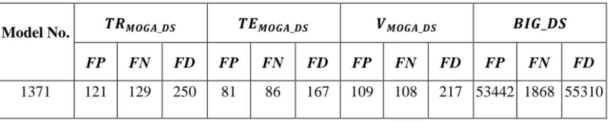
Table IV shows the models whose False Positive and False Negative rates are less than 3% in 𝐵𝐼𝐺_𝐷𝑆. As it can be seen, both models have an equal percentage of FP (i.e., 2.96%) within 𝐵𝐼𝐺_𝐷𝑆 but the FN percentage of model 1371 within 𝐵𝐼𝐺_𝐷𝑆 is slightly smaller than that of model 6009. Hence, the statistics of model 1371, shown in Table V, were used as restrictions on experiment 2.

Table IV. Models of experiment 1 whose False Positive and False Negative rates are less than 3% in 𝐵𝐼𝐺_𝐷𝑆

Model No. 𝑻𝑹𝑴𝑶𝑮𝑨_𝑫𝑺 𝑻𝑬𝑴𝑶𝑮𝑨_𝑫𝑺 𝑽𝑴𝑶𝑮𝑨_𝑫𝑺 𝑩𝑰𝑮_𝑫𝑺 𝑴𝑪

FP (%) FN (%) FD (%) FP (%) FN (%) FD (%) FP (%) FN (%) FD (%) FP (%) FN (%) FD (%)

1371 0.80 2.70 1.25 2.43 2.58 2.51 3.27 3.24 3.26 2.96 2.88 2.96 702 6009 0.74 2.53 1.17 2.85 2.46 2.66 3.36 3.06 3.21 2.96 2.89 2.96 870

Table V. Statistics of model 1371.

Model No. 𝑻𝑹𝑴𝑶𝑮𝑨_𝑫𝑺 𝑻𝑬𝑴𝑶𝑮𝑨_𝑫𝑺 𝑽𝑴𝑶𝑮𝑨_𝑫𝑺 𝑩𝑰𝑮_𝑫𝑺

FP FN FD FP FN FD FP FN FD FP FN FD

1371 121 129 250 81 86 167 109 108 217 53442 1868 55310

Experiment 2 resulted in 281non-dominated models from which 69 models are in the preferable set. Table VI shows the Minimum, Average and Maximum FP and FN rates as well as the model complexity over this set. Table VII shows the preferable models of experiment 2 whose FP and FN rates are less than 2.6% in 𝐵𝐼𝐺_𝐷𝑆. Analyzing the results of Table VII, one can see that

employing restrictions on 𝐹𝑁_𝑇𝑅 and 𝐹𝑃_𝑇𝑅 resulted in models with smaller number of false detections in all sets, including in BI𝐺_𝐷𝑆. Among the models in Table VII, model 3726 has the minimum percentage of FP and model 3055 has the minimum percentage of FN on 𝐵𝐼𝐺_𝐷𝑆.

Table VI. Min, Avg. and Max false positive and false negative rates as well as model complexity of 69 models in the preferable set of experiment 2.

𝑻𝑹𝑴𝑶𝑮𝑨_𝑫𝑺 𝑻𝑬𝑴𝑶𝑮𝑨_𝑫𝑺 𝑽𝑴𝑶𝑮𝑨_𝑫𝑺 𝑩𝑰𝑮_𝑫𝑺 _𝑴𝑪

FP (%) FN (%) FD (%) FP (%) FN (%) FD (%) FP (%) FN (%) FD (%) FP (%) FN (%) FD (%)

Min. 0.49 1.38 0.77 2.19 2.06 2.36 2.24 1.75 2.05 2.40 1.98 2.40 750

Avg. 0.60 1.90 0.89 2.76 2.65 2.71 2.71 2.45 2.58 2.78 2.43 2.76 862.3

Max. 0.67 2.51 1.04 3.37 3.37 3.25 3.24 2.97 2.97 3.20 2.91 3.17 900

Table VII. Preferable models of experiment 2 whose false positive and false negative rates are less than 2.6% in 𝐵𝐼𝐺_𝐷𝑆 Model No. 𝑻𝑹𝑴𝑶𝑮𝑨_𝑫𝑺 𝑻𝑬𝑴𝑶𝑮𝑨_𝑫𝑺 𝑽𝑴𝑶𝑮𝑨_𝑫𝑺 𝑩𝑰𝑮_𝑫𝑺 _𝑴𝑪 FP (%) FN (%) FD (%) FP (%) FN (%) FD (%) FP (%) FN (%) FD (%) FP (%) FN (%) FD (%) 3726 0.60 1.79 0.87 2.27 2.90 2.58 2.58 2.37 2.48 2.40 2.34 2.40 870 4812 0.60 1.87 0.89 2.71 2.30 2.50 2.61 2.71 2.66 2.60 2.43 2.59 900 3863 0.59 1.52 0.80 2.32 2.71 2.52 2.43 2.56 2.49 2.55 2.45 2.55 900 3055 0.50 1.73 0.77 2.71 2.84 2.78 2.43 2.09 2.26 2.56 2.31 2.55 900

6.3 Ensemble of models in the preferable set of experiment 2

Having selected a model (model 3726 shown in Table VII) with acceptable rates of specificity 97.60% (i.e., 2.40 % FP rate) and sensitivity 97.66% (i.e., 2.34% FN rate) at pixel level, an ensemble of the preferable models obtained in experiment 2 was also considered as a classifier. Each data sample is fed to all 69 preferable models and then a majority vote determines whether the pixel is considered normal or abnormal. Table VIII shows the results obtained on 𝑀𝑂𝐺𝐴_𝐷𝑆 and 𝐵𝐼𝐺_𝐷𝑆. Comparing the results with the ones obtained from model 3726 in Table VII, it can be seen that 0.41% and 0.56% reductions could be obtained in the FP and FN rates over 𝐵𝐼𝐺_𝐷𝑆,

respectively. Hence, the ensemble approach achieves a specificity of 98.01% (i.e., 1.99 % FP rate) and a sensitivity of 98.22% (i.e., 1.78% FN rate) at pixel level over 𝐵𝐼𝐺_𝐷𝑆.

Table VIII. Results of the ensemble of preferable models of experiment 2 on 𝑀𝑂𝐺𝐴_𝐷𝑆 and 𝐵𝐼𝐺_𝐷𝑆 Ensemble of preferable models in experiment 2 𝑻𝑹𝑴𝑶𝑮𝑨_𝑫𝑺 𝑻𝑬𝑴𝑶𝑮𝑨_𝑫𝑺 𝑽𝑴𝑶𝑮𝑨_𝑫𝑺 𝑩𝑰𝑮_𝑫𝑺 FP (%) FN (%) FD (%) FP (%) FN (%) FD (%) FP (%) FN (%) FD (%) FP (%) FN (%) FD (%) 0.44 1.18 0.61 1.90 2.03 1.96 1.93 1.74 1.83 1.99 1.78 1.99

6.4 Visualizing abnormal regions in CT images using the ensemble of preferable models

Figure 11 shows the results of applying the ensemble of preferable models on some CT images, where the output images of the classifier were marked with different colors, depending on the classifier output for each tested pixel. The color code is shown in Table IX.

Table IX. Colour code used for marking pixels based on the percentage of preferable models with a positive output

Percentage of preferable models with a positive output

Colour code Description

[66% 100%] Red Clear presence of pathology [50% 66%) Blue Cannot decide whether the

pixel is normal or abnormal [0% 50%) --- Clear absence of pathology

(d) (e) (f)

(g) (h) (i)

Figure 11. The result of applying the ensemble of preferable models on CT images. (a), (d) and (g) are the original images. (b), (e) and (h) are marked by the Neuroradialogist. (c), (f) and (i) are

marked by the classifier.

6.5 Features use

To understand which features are the most frequent in the preferable models of experiment 2, the relative frequency of each feature 𝑓𝑖 within the 69 models is shown in Figure 12. One can see that, among the allowable 30 features within the 51 features considered, features {𝑓2, 𝑓4, 𝑓5, 𝑓7, 𝑓12, 𝑓33, 𝑓41, 𝑓42, 𝑓44, 𝑓45 } are the ones that have been employed in more than 80% of the models. Among this set, features {𝑓2, 𝑓4, 𝑓5, 𝑓7, 𝑓12, 𝑓41 } belong to the set of first order statistics, feature 𝑓33 is a second order statistic and features {𝑓42, 𝑓44, 𝑓45} are symmetry features.

Figure 12. Relative frequency of each feature in the preferable models of experiment 2.

7. Discussion

As was shown before, the proposed approach achieves an excellent performance, both in terms of sensitivity and specificity. Moreover, as it is a pixel-based classifier, lesion contours are obtained, very close to the ones marked by the Neuroradiologist. A comparison of this approach with other works is, however, difficult as, to the best of our knowledge, there is no alternative system that uses a pixel-based classification.

As Support Vector Machines (SVM) are frequently used in classification purposes, in the next subsection we change our model, a MOGA-designed RBFNN to a SVM, and compare its use as a pixel-based classifier. The subsequent subsection will compare the proposed approach with three existing alternatives found in the literature. As pointed out before, these systems work at a slice level, which means that they can identify lesions but not draw their contours.

7.1 Comparing MOGA RBF classifiers with Support Vector Machines

In order to compare the obtained results with a SVM [39], the MATLAB SVM tool with Gaussian RBF (Radial Basis Function) kernel was used. For determining the best penalty parameter (C) and the spread, 121 possible combinations obtained by selecting 2 values from the set {0.003, 0.01, 0.03, 0.1, 0.3, 1, 3, 10, 30, 100, 300} were used for SVM training, and the combination (C=3, spread=1) whose error on the test set was minimum, was selected. In this experiment, 69.8% of the data samples in the training set were considered as support vectors. Table X shows the FP and FN rates when this SVM was applied.

Comparing the results with the ones obtained with the ensemble of models, shown in Table VIII, and also with model 3726, shown in Table VII, one can see that even with a huge complexity of the SVM model (139,600 support vectors), its FP and FN rates in 𝐵𝐼𝐺_𝐷𝑆 are not only higher than the ones obtained with the ensemble of preferable models, but also the ones achieved by model

3726. Notice that a SVM model, with Gaussian Kernel can be considered a RBFNN model, where the centers of the Gaussians are the support vectors, and with a common spread to all the neurons. In this case, all the features (51) were considered as inputs and 13960 support vectors were employed. This is translated into a complexity of 711,960 parameters, determined by the SVM algorithm. This figure should be compared with a complexity of 870 (around 0.1%), for model 3726 in Table VII.

Table X. FP and FN rates using SVM

𝑇𝑅𝑀𝑂𝐺𝐴_𝐷𝑆 𝑇𝐸𝑀𝑂𝐺𝐴_𝐷𝑆 𝑉𝑀𝑂𝐺𝐴_𝐷𝑆 𝐵𝐼𝐺_𝐷𝑆

FP (%) FN (%) FD (%) FP (%) FN (%) FD (%) FP (%) FN (%) FD (%) FP (%) FN (%) FD (%)

0.16 0 0.13 2.6 2.42 2.51 2.32 2.26 2.29 2.5 2.37 2.5

7.2 Comparing the results obtained with other approaches

The authors in [40] presented a Computer Aided Detection (CAD) method for early detection of CVAs from CT images where, in the same way as this work, in a preprocessing phase artifacts are removed and tilted CT images are realigned. In order to find the regions that have higher probability of being considered lesions, a Circular Adaptive Region Of Interest (CAROI) algorithm is applied on each CT slice, which aims to draw a circular border around areas with sudden change of intensity values. Each circular region is then compared with its corresponding region in the other side of the brain using the Pearson correlation coefficient. Those circular areas which have the smallest PCC values are selected for further investigation. Eight second order features are calculated from the GLCM matrix of previously selected circular regions and are passed to a 3-layer feed-forward back propagation neural network which was trained using 10 normal and 20 abnormal cases in a round robin (leave-one-out) fashion. The output of neural network identifies whether the circular region is a lesion or not.

In order to evaluate their CAD system, 31 positive cases containing 82 ischemic strokes (39 acute and 43 chronic) were used as validation set. A sensitivity of 76.92% (i.e., 30/39 lesion areas correctly detected) for acute ischemic strokes and a sensitivity of 90.70% (i.e., 39/43 lesion areas correctly detected) for chronic strokes were reported. This gives a total sensitivity of 84.14% (i.e.,

30+39

82 × 100).

In spite of the differences of this approach and ours, in order to be able to compare the accuracy obtained in terms of lesions sensitivity, this measure has been calculated. A total number of 35 ischemic lesions within 150 CT images were marked by our collaborating Neuroradiologist. The ensemble of preferable models in experiment 2 detected 30 lesions correctly, which is translated in a sensitivity of 85.71%, slightly higher than approach [40].

The authors in [41] developed a CAD system for detecting hemorrhagic strokes in CT images. After removing the artifacts and realigning the tilted images, the hemorrhagic areas are segmented by employing a threshold on the pixels’ intensity values. To detect the edema regions, a higher contrast ratio of a given CT image is firstly obtained using a local histogram equalization. A thresholding method is then applied to segment the edema region from the normal tissue. The accuracy of the CAD system is evaluated by comparing the area of bleeding region (ABR) and edema region (AER) that are detected by the CAD and the ones that are marked by the doctor using data from 8 spontaneous hemorrhagic stroke patients. It is reported that the average difference of ABRs is 8.8%, and the average of the degree of coincidence is 86.4%, while the average difference of AERs is 14.1%, with an average of degree of coincidence of 77.4%.

The results obtained by this approach cannot be exactly compared with the approach presented here, as [41] deals with hemorrhagic strokes, which typically are much easier to detect and mark than ischemic strokes. In spite of that, the average difference of the areas as well as the average degree of coincidence have been computed for the cases presented here, for the lesions both marked by the doctor and detected by our system. The average difference is 11.4%, and the average degree of coincidence is 88.6%. These figures are better than the values obtained for AER, in approach [41].

The authors in [42] utilize a combination of 2D and 3D Convolutional Neural Networks (CNN) to cluster brain CT images into 3 groups: Alzheimer’s disease, lesion and normal ageing. The best classification accuracy rates using the proposed CNN architecture are 85.2%, 80% and 95.3% for the classes of Alzheimer’s disease, lesion and normal, respectively, with an average of 87.6%. To be able to compare the classification accuracy rates of our work with the ones in [42], we calculated this metric in a CT slice level, by labeling each CT slice as normal or abnormal (i.e., having one or more lesions). Our system was able to correctly identify all 24 CT slices that had lesions within which translates into 100% classification accuracy rate for the abnormal group. Among the remaining 126 normal CT slices, our system identified small false lesions within 7 CT slices, which means that we obtained a 94.4 % classification accuracy rate for the normal group.

8. Conclusions

In this work, a RBFNN based system for automatic identification of CVA through the analysis of brain CT images is presented. Considering a set of 51 features, the MOGA design framework was employed to find the best possible RBFNN structure and its corresponding parameters. Two experiments were conducted in MOGA. The best result is obtained from an ensemble of preferable models of experiment 2, where the 𝐹𝑁_𝑇𝑅 and 𝐹𝑃_𝑇𝑅 objectives were restricted based on the results obtained by the best model from the first experiment. Values of specificity of 98.01% (i.e., 1.99 % FP) and sensitivity of 98.22% (i.e., 1.78% FN) were obtained at pixel level, in a set of 150 CT slices (1,867,602 pixels).

Comparing the classification results with SVM over 𝐵𝐼𝐺_𝐷𝑆, despite the huge complexity of the SVM model, the accuracy of the selected model in experiment 2, as well as the ensemble of preferable models, are superior to that of SVM model.

The present approach compares also favorably with other similar published approaches, achieving improved sensitivity at lesion level than [40], better average difference and degree of coincidence than [41], as well as superior classification accuracy rate than [42]. It should be stressed than none of these methods are able to draw the lesion(s) contour(s), as it is achieved by the proposed approach.

As the number of abnormal pixels is much smaller than the number of normal pixels in the existing dataset, at the present stage the classifier is able to detect the great majority of the lesions, but sometimes will identify false lesions. Current research is tackling this problem. Additionally, as the proposed classifier was designed and tested only with CT images including ischemic CVAs, we consider enlarging the CT database to include other brain lesions, and apply the same methodology to design an additional classifier capable of discriminating brain lesions with similar image patterns.

Acknowledgments

The authors would like to acknowledge the support of FCT, through IDMEC, under LAETA, project UID/EMS/50022/2013 and Dr. Luis Cerqueira, from Centro Hospitalar de Lisboa Central, Portugal, for marking the exams.

References

[1] A. S. Go, D. Mozaffarian, V. L. Roger, E. J. Benjamin, J. D. Berry, W. B. Borden, et al., "Heart disease and stroke statistics--2013 update: a report from the American Heart Association," Circulation, vol. 127, pp. e6-e245, Jan 1 2013.

[2] P. M. Ferreira and A. E. Ruano, "Evolutionary Multiobjective Neural Network Models Identification: Evolving Task-Optimised Models," New Advances in Intelligent Signal

Processing, vol. 372, pp. 21-53, 2011.

[3] E. Hajimani, M. G. Ruano, and A. E. Ruano, "MOGA design for neural networks based system for automatic diagnosis of Cerebral Vascular Accidents," in 9th IEEE

International Symposium on Intelligent Signal Processing (WISP), 2015, pp. 1-6.

[4] E. Hajimani, A. Ruano, and G. Ruano, "The Effect of Symmetry Features on Cerebral Vascular Accident Detection Accuracy," presented at the RecPad 2015, the 21th edition of the Portuguese Conference on Pattern Recognition, Faro, Portugal, 2015.

[5] X. Llado, A. Oliver, M. Cabezas, J. Freixenet, J. C. Vilanova, A. Quiles, et al., "Segmentation of multiple sclerosis lesions in brain MRI: A review of automated approaches," Information Sciences, vol. 186, Mar 1 2012.

[6] T. Hachaj and M. R. Ogiela, "CAD system for automatic analysis of CT perfusion maps,"

Opto-Electronics Review, vol. 19, Mar 2011.

[7] L. E. Poh, V. Gupta, A. Johnson, R. Kazmierski, and W. L. Nowinski, "Automatic Segmentation of Ventricular Cerebrospinal Fluid from Ischemic Stroke CT Images,"

Neuroinformatics, vol. 10, Apr 2012.

[8] W. L. Nowinski, G. Qian, K. N. B. Prakash, Q. Hu, and A. Aziz, "Fast Talairach Transformation for magnetic resonance neuroimages," Journal of Computer Assisted

Tomography, vol. 30, pp. 629-641, Jul-Aug 2006.

[9] N. Otsu, "A Threshold Selection Method From Gray-level Histogram," IEEE

Transactions on Systems, Man, and Cybernetics, 1978.

[10] M. Gao and S. Chen, "Fully Automatic Segmentation of Brain Tumour in CT Images,"

European Journal of Cancer, vol. 47, Sep 2011.

[11] A. P. Nanthagopal and R. S. Rajamony, "Automatic classification of brain computed tomography images using wavelet-based statistical texture features," Journal of

Visualization, vol. 15, pp. 363-372, Nov 2012.

[12] T. J. Devadas and R. Ganesan, "Analysis of CT Brain images using Radial Basis Function Neural Network," Defence Science Journal, vol. 62, Jul 2012.

[13] O. Freifeld, H. Greenspan, and J. Goldberger, "Lesion detection in noisy MR brain images using constrained GMM and active contours," 4th IEEE International Symposium

on Biomedical Imaging : Macro to Nano, Vols 1-3, pp. 596-599, 2007.

[14] H. Greenspan, A. Ruf, and J. Goldberger, "Constrained Gaussian mixture model framework for automatic segmentation of MR brain images," IEEE Transactions on

Medical Imaging, vol. 25, pp. 1233-1245, Sep 2006.

[15] B. J. Bedell and P. A. Narayana, "Automatic segmentation of gadolinium-enhanced multiple sclerosis lesions," Magnetic Resonance in Medicine, vol. 39, pp. 935-940, Jun 1998.

[16] A. O. Boudraa, S. Mohammed, R. Dehak, Y. M. Zhu, C. Pachai, Y. G. Bao, et al., "Automated segmentation of multiple sclerosis lesions in multispectral MR imaging using fuzzy clustering," Computers in Biology and Medicine, vol. 30, pp. 23-40, Jan 2000.

[17] E. Hajimani, C. A. Ruano, M. G. Ruano, and A. E. Ruano, "A software tool for intelligent CVA diagnosis by cerebral computerized tomography," in 8th IEEE

International Symposium on Intelligent Signal Processing (WISP), 2013, pp. 103-108.

[18] X. Qi, A. Belle, S. Shandilya, W. Chen, C. Cockrell, Y. Tang, et al., "Ideal Midline Detection Using Automated Processing of Brain CT Image," Open Journal of Medical

Imaging, vol. 3, p. 9, 2013.

[19] L. He, Y. Chao, K. Suzuki, and K. Wu, "Fast connected-component labeling," Pattern

Recognition, vol. 42, pp. 1977-1987, Sep 2009.

[20] A. Usinskas, R. A. Dobrovolskis, and B. F. Tomandl, "Ischemic stroke segmentation on CT images using joint features," Informatica, vol. 15, pp. 283-290, 2004.

[21] L. Ribeiro, A. E. Ruano, M. G. Ruano, and P. M. Ferreira, "Neural networks assisted diagnosis of ischemic CVA's through CT scan," IEEE International Symposium on

Intelligent Signal Processing, Conference Proceedings Book, pp. 223-227, 2007.

[22] W. Chen, R. Smith, S.-Y. Ji, K. R. Ward, and K. Najarian, "Automated ventricular systems segmentation in brain CT images by combining low-level segmentation and