Universidade do Minho Escola de Engenharia Departamento de Inform´atica
Pedro Emanuel Silva Ferreira
AIoTA
An IoT Platform On MonetDB
Universidade do Minho
Escola de Engenharia Departamento de Inform´atica
Pedro Emanuel Silva Ferreira
AIoTA
An IoT Platform On MonetDB
Master dissertation
Master Degree in Computer Science
Dissertation supervised by
Dr. Jos ´e Orlando Roque Nascimento Pereira Dr. Ying Zhang
A C K N O W L E D G M E N T S
This thesis is the final step on my masters graduation, and I would to thank several people who helped me during my academic career and the thesis itself. It also brought me the opportunity to do an Erasmus traineeship, which will be my first experience abroad.
I want to thank to the academic community of University of Minho for my formation during the past 5 years. For the most, I am thankful to Dr. Jos´e Orlando Pereira for his acceptance to be my supervisor during the thesis, his knowledge about database systems that helped me during this report, his availability and the opportunity he gave to me for the internship at CWI on the second semester. Also I want to thank the personnel from Distributed Systems at University of Minho and HASLab groups for their accommodation. This thesis could not be done without the help of the community of Database Archi-tectures group from CWI, who I want to thank deeply. First I want to thank Dr. Stefan Manegold for writing my acceptance letter to the Erasmus traineeship. Next I want to appraise the MonetDB Solutions personnel from the group for their help during AIoTA conception: Panagiotis Koutsourakis, Dimitar Nedev, Dr. Hannes M ¨uhleisen, Dr. Sjoerd Mullender and Dr. Niels Nes. A special thanks to Abe Wits, Mrunal Gawade, Pha.m Minh D ´uc and Bo Tang for the great moments we shared together in our office. At the same time I want to thank Till D ¨ohmen, Benno Kruit, Mark Raasveldt, Dean De Leo, Thibault Sellam, Eleni Petraki, Dr. Bart Scheers, Dr. Romulo Gonc¸alves and Dr. Eyal Rozenberg for amazing moments during the internship sharing knowledge and happiness.
Meanwhile, another special thanks from the service staff from CWI that help me on the internship. Irma van Lunenburg for her help and availability during my CWI registration. Bikkie Aldeias, Martine Gunzeln and Minnie Middelberg for their help during my first days at CWI. Arjen de Rijke for his help during IT-related installations.
I want to express greater gratitude to my supervisor at CWI Dr. Ying Zhang for her supervision, knowledge about database systems and hospitality. At the same time I want to give appreciation to Dr. Martin Kersten as the founder of the group and MonetDB, who helped building the back-end of AIoTA. Without his help, this thesis would not be able to finish on time.
In the end, I want to send cheers for my family, especially my parents, who raised and taught me during my whole life. Without their help, I could never accomplish this. Also it could not be done with the help of my local living community of Tadim and my friends, to whom I express gratitude.
A B S T R A C T
The growth of the Internet and embedded systems have allowed physical devices to collect and exchange data in the Internet-of-Things (IoT). IoT allows objects to be monitored and controlled remotely across an existing network infrastructure, while creating opportunities to assimilate computer systems with the real world. The expansion of IoT’s connectivity has lead devices to exchange large amounts of data, due to constantly required monitoring. The output of these devices can be seen as streams with data made available incrementally over time. This has created a new demand to collect, process and analyze IoT data in an efficient and scalable way.
In the meantime, databases have been organizing collections of data for several decades. At a low level, database management systems (DBMSs) to organize data efficiently. In par-ticular, Data Stream Management Systems (DSMSs) have emerged to handle uninterrupted flows of streaming data and integrate them with relational databases [Aggarwal, 2007]. With this objective in mind, DSMSs have distinguished from traditional DBMSs with new architectures, data models, algorithms and specific query languages to deal with streams. As streams are uninterrupted, DSMSs aim to process them incrementally. This lead to the continuous queries concept, where streaming data is processed with small batches each time.
Meanwhile, other database management systems have explored alternate ways to orga-nize data. MonetDB is a pioneer column-oriented relational database management sys-tem (RDBMS), storing relations column-wise opposed to rows as the majority of RDBMSs. Columnar-wise storage allows several benefits such as per-column query parallelization, data compression and late materialization. MonetDB is being developed at Centrum Wiskunde & Informatica (CWI) in Amsterdam since 1993, having achieved faster benchmark results than popular RDBMSs such as PostgreSQL [Muhleisen,2014].
This master thesis has the objective to create a streaming engine over MonetDB while focusing on IoT processing. Amsterdam Internet-of-Things App (AIoTA) is a full-stack application aiming to be integrated easily with IoT devices to collect streaming data, while taking advantage of MonetDB’s columnar-wise storage to process it and deliver results immediately.
R E S U M O
O crescimento da Internet e dos sistemas embebidos tem permitido expor dispositivos f´ısicos na Internet das coisas (IoT) para a troca de dados. A IoT permite a monitorizac¸˜ao de objetos remotamente em infraestruturas de rede criando oportunidades para assimilar a computac¸˜ao com o mundo real. A expans˜ao da conetividade da IoT tem levado esses dispositivos a promover o intercˆambio de grandes quantidades de dados, em maior parte devido a monitorizac¸˜ao constante. Os dados resultantes desses dispositivos podem ser visto como streams, onde os dados s˜ao disponibilizados incrementalmente com o decorrer do tempo. Como consequˆencia, as streams criaram uma nova forma de colecionar, processar e analisar dados provenientes da IoT de modo eficiente e escal´avel.
Ao mesmo tempo nas ´ultimas d´ecadas, as bases de dados tem organizado colec¸ ˜oes de dados. A um n´ıvel mais baixo, os sistemas de gest˜ao de bases de dados (DBMSs) tem procu-rado metodologias para organizar os dados de forma eficiente. Em particular, os sistemas de gest˜ao de streams (DSMSs) tem emergido com novos m´etodos para lidar com fluxos de dados inenterruptos e integr´a-los com as bases de dados convencionais [Aggarwal,2007]. Com este objetivo em mente, as DSMSs tem-se distinguido dos DBMSs com novas arquite-turas, modelos de dados, algoritmos e linguagens de interrogac¸˜ao para lidar com streams. Como as streams s˜ao inenterruptas, as DSMSs tem a finalidade de as processar incremen-talmente. Isto levou ao conceito de continuous queries, onde as streams so processadas com pequenas quantidades de cada vez e incrementalmente.
Entretanto outros sistemas de gest˜ao de bases dados tem explorado metodologias al-ternativas para organizar os dados. O MonetDB ´e um sistema de gest˜ao de bases dados relacional colunar pioneiro, onde as relac¸ ˜oes s˜ao armazenadas por colunas em vez de linhas como a maioria dos RDBMSs. O armazenamento colunar permite v´arios benef´ıcios que n˜ao seriam poss´ıveis com o armazenamento por linhas tais como paralelizac¸˜ao de interrogac¸ ˜oes por colunas, compress˜ao de dados e materilizac¸˜ao mais tardia. O MonetDB tem sido de-senvolvido pelo Centrum Wiskunde & Informatica (CWI) em Amsterd˜ao desde 1993, tendo alcanc¸ado benchmarks com melhores resultados em comparac¸˜ao com populares sistema de gest˜ao de bases dados como o PostgreSQL [Muhleisen,2014].
Esta tese de mestrado tem o objetivo de criar uma extens˜ao de streaming no MonetDB com focus na IoT. A Amsterdam Internet-of-Things App (AIoTA) ´e uma aplicac¸˜ao full-stack com o objetivo de ser integrada facilmente com dispositivos IoT para colecionar dados para streams, tendo ao mesmo tempo como vantagem o armazenamento colunar do MonetDB para processar os dados e disponibilizar resultados imediatamente.
C O N T E N T S
1 i n t r o d u c t i o n 1
1.1 Contextualization 1
1.2 Problem Statement 2
1.3 Objective 2
1.4 Structure of the Document 3
2 r e l at e d w o r k 4
2.1 Motivation for Streaming Systems 4
2.2 Real Life Applications of Streaming 5
2.3 Programming Models 6
2.4 Streaming Query Languages 7
2.5 Windows 8
2.6 Streaming Operators and Continuous Queries 10
2.7 Time and Order 11
2.7.1 Timestamps 11
2.7.2 Order 12
2.8 Query Optimizations 13
2.9 Streaming Engines Outline 15
2.9.1 Apache Storm 15
2.9.2 Apache Spark Streaming 16
2.9.3 PipelineDB 17 2.9.4 DataCell 18 3 m o n e t d b ov e r v i e w 19 3.1 Column-wise Storage 19 3.2 Internal Representation 20 3.3 Query Processing 21 4 a i o ta p l at f o r m 23 4.1 Design Considerations 23
4.2 AIoTA Architecture Overview 24
4.3 AIoTA Workflow 25
5 i o t w e b s e r v e r i m p l e m e n tat i o n 26
5.1 RESTful Systems 26
5.2 IoT Web Server Bootstrap 27
5.3 IoT Web Server Life-Cycle 28
Contents v
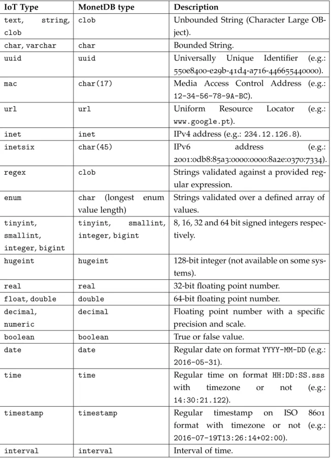
5.4 Data Types Mapping 29
5.5 RESTful API 31
6 w e b a p i s e r v e r i m p l e m e n tat i o n 32
6.1 WebSockets Protocol 32
6.2 Web API Server Bootstrap 33
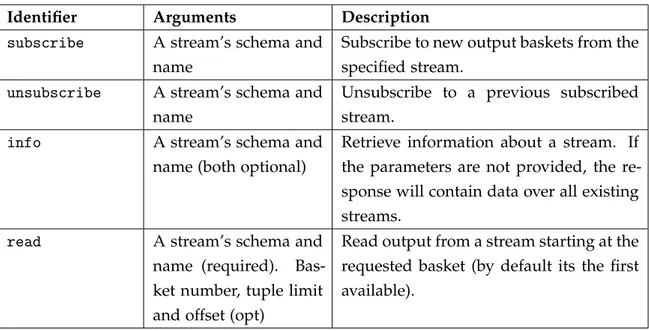
6.3 WebSockets API 33
7 m o n e t d b s t r e a m i n g e n g i n e i m p l e m e n tat i o n 35
7.1 Scheduler 35
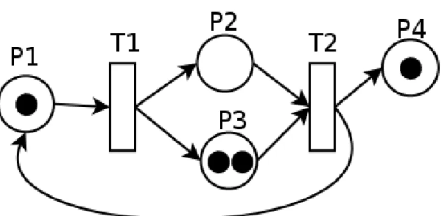
7.1.1 Petri-net model 36
7.1.2 Continuous queries scheduler 37
7.1.3 Concurrent continuous queries 37
7.2 SQL Catalog 39
7.2.1 Scheduling procedures 39
7.2.2 Windowing functions and procedures 40
7.2.3 Baskets procedures 41
7.2.4 Debugging functions and procedures 41
7.2.5 SQL catalog example 42
7.3 Aggregations on Continuous Queries 44
7.4 Continuous Query Plans and Optimizations 45
7.4.1 New iot optimizer 46
7.4.2 Query execution comparison 46
8 e va l uat i o n 49
8.1 Functional Evaluation 49
8.1.1 Stream processing requirements 49
8.1.2 Comparison against the state of the art 52
8.2 Performance Evaluation 55
8.2.1 Flame Graphs on the web servers 55
8.2.2 Tomograph on the streaming engine 61
8.2.3 AIS benchmarking tests 63
9 c o n c l u s i o n a n d f u t u r e w o r k 70
9.1 Conclusion 70
9.2 Future Work 71
a i o t w e b s e r v e r i m p l e m e n tat i o n d e ta i l s 80
a.1 Server Arguments 80
a.2 Supported Data Types 81
a.3 RESTful API 84
Contents vi a.3.2 Application Server 86 b w e b a p i s e r v e r i m p l e m e n tat i o n d e ta i l s 88 b.1 Server arguments 88 b.2 WebSockets API 89 b.2.1 Requests 89 b.2.2 Responses 90 c m o n e t d b s t r e a m i n g e n g i n e i m p l e m e n tat i o n d e ta i l s 94
c.1 Final MAL Execution Plans 94
c.1.1 Regular table 94 c.1.2 Streaming table 96 d a i s b e n c h m a r k q u e r i e s 98 d.1 AIoTA Queries 98 d.1.1 AIS query 1 99 d.1.2 AIS query 3 99 d.1.3 AIS query 11 99 d.2 PipelineDB queries 100 d.2.1 AIS query 1 100 d.2.2 AIS query 3 100 d.2.3 AIS query 11 101
L I S T O F F I G U R E S
Figure 1 Query processing comparison between DBMSs and DSMSs. 5 Figure 2 Comparison of some windows implementations in data streams. 10 Figure 3 Operators’ arrangements for Chain scheduling. 14 Figure 4 Internal representation of row and columnar wise storage. 19 Figure 5 MonetDB’s components and relations during the execution of a SQL
query. 22
Figure 6 AIoTA’s proposed platform, components and relations. 24 Figure 7 A Petri-net graphical representation. 37 Figure 8 The concurrency problem solution through a Petri-net 38 Figure 9 Flame Graph corresponding to creating a stream at IoT Web Server. 57 Figure 10 Flame Graph corresponding to make a 1000 tuple batch insert at IoT
Web Server. 58
Figure 11 Flame Graph corresponding to read 1000 tuples from a Output
Bas-ket at IoT Web API. 59
Figure 12 Result tomograph from temperature examination continuous query. 62 Figure 13 Evolution of average Latency and Throughput for AIS query 1 with
the number of clients. 67
Figure 14 Evolution of average latency and throughput for AIS query 3 with
the number of clients. 67
Figure 15 Evolution of average latency and throughput for AIS query 11 with
the number of clients. 68
L I S T O F TA B L E S
Table 1 Comparison between a DBMS and a DSMS. In the general scenario, DSMSs behave in a more stochastic environment than DBMSs. 5 Table 2 IoT Web Server supported data types and correspondent MonetDB
mappings. 30
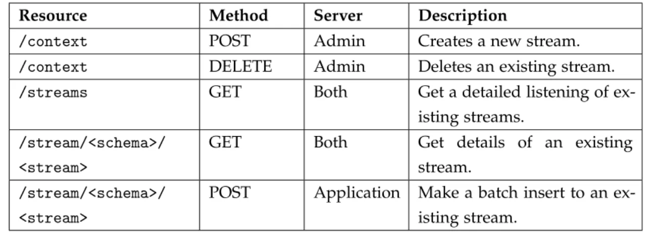
Table 3 Available resources on IoT Web Server’s RESTful API. 31 Table 4 Available IoT Web API WebSocket requests. 34 Table 5 Available IoT Web API WebSocket responses. 34 Table 6 Available scheduling procedures in the SQL catalog. 39 Table 7 Available windowing procedures and functions in the SQL
cata-log. 40
Table 8 Available baskets procedures in the SQL catalog. 41 Table 9 Available debugging procedures and functions in the SQL catalog. 42 Table 10 Functional comparison between AIoTA and PipelineDB. 54
Table 11 AIS benchmark queries. 66
1
I N T R O D U C T I O N1.1 c o n t e x t ua l i z at i o n
The Internet-of-Things (IoT) allows objects to be sensed and controlled remotely across an existing network infrastructure, while creating opportunities to assimilate computer sys-tems with the real world. With IoT, it is possible to change the way people interact with objects for a better quality of life. In 2011 there was about 25 billion devices connected to IoT, and by 2020 that number is expected to double [Evans, 2011]. The IoT’s applicability is very wide, from health care and home monitoring, to agriculture and car vigilance. In this way the market of IoT is growing significantly as both consumers and businesses are getting benefits from connecting devices to the Internet [Greenough,2014].
The expansion of IoT’s connectivity has lead devices to exchange large amounts of data, due to constantly required monitoring. The output of these devices can be seen as streams with data made available incrementally over time. As a consequence, IoT accommodates the Big Data model which translates into data that needs to be processed efficiently from many sources simultaneously, while producing results promptly.
Big Data is often defined by the 4 V’s: Volume, Variety, Velocity and Veracity [Han and Lu, 2014]. Volume represents the quantity of data, its size determines the value and potential of the data. Variety describes the possible types of data and the sources they can come from. Velocity indicates the speed that the data is being generated and the quickness of processing required to the demand. Finally Veracity represents the quality of the final results and how much efficiently we can process data without declining the quality. Due to these reasons, IoT and other stream-based applications such as social networks, lead to research focusing on large scale and high availability technologies for Big Data. This demand ranges from subjects such as machine learning and data mining, to scalability and data management.
Databases have been organizing collections of data for several decades. At a higher level, Database Management Systems (DBMSs) have researched how to organize data efficiently and have explored new ways to collect it simultaneously. In particular, Data Stream Man-agement Systems (DSMSs) have emerged to research new methodologies on how to handle with uninterrupted flows of streaming data and integrate them with relational databases
1.2. Problem Statement 2 [Aggarwal,2007]. With this objective in mind, DSMSs have distinguished from traditional with new architectures, data models, algorithms and specific query languages to deal with streams. As streams are uninterrupted, DSMSs aim to process them incrementally. This lead to the continuous queries concept, where streaming data is processed with small batches each time.
Meanwhile, other DBMSs have explored alternate ways to organize data. MonetDB is a pioneer column-oriented relational database management system (RDBMS), storing rela-tions column-wise opposed to rows as the majority of RDBMSs. Columnar-wise storage allows several benefits not capable row-wise such as column caching, data compression and late materialization of the results. MonetDB is being developed at Centrum Wiskunde & Informatica (CWI) in Amsterdam since 1993, takes full support of the ACID properties [CWI, 2015] and compiles the 2003 SQL standard. Through the years, MonetDB has re-searched new ways to build large scale databases in a more efficiently and scalable way, while taking advantage of column-wise storage [Idreos et al., 2012]. This research made MonetDB achieve faster TPC-H results than popular row-oriented RDBMSs such as Post-greSQL [Muhleisen,2014].
1.2 p r o b l e m s tat e m e n t
To accommodate the IoT interest raise in Amsterdam city in the last years, along with special attention to the recently proposed Amsterdam IoT network [de Vries, 2015], this report details the creation process of Amsterdam Internet-of-Things App (AIoTA), a new streaming application developed for MonetDB. This application has the objective to create a DSMS on MonetDB while focusing on IoT processing and fulfilling the Big Data 4 V’s as much as possible. AIoTA is a full stack application aiming to be integrated easily with IoT devices to collect streaming data, while taking advantage of MonetDB’s columnar-wise storage to process it and deliver results promptly.
1.3 o b j e c t i v e
The main objective of this master thesis is to add a flexible streaming engine to AIoTA with focus on Internet-of-Things processing. For the IoT devices, two web servers will be created (one to input data and other for output data), hence the database layer will be completely transparent for them. As the DSMSs’ implementation is quite divergent in the market, we will extend the MonetDB’s kernel code with a simple but flexible streaming engine aiming to cover many of the existing solutions in the market.
1.4. Structure of the Document 3 1.4 s t r u c t u r e o f t h e d o c u m e n t
In Chapter 2, a research of related work in DSMSs is conducted. In this Chapter the evo-lution of DSMSs, their motivation and challenges are reported. At its end, some of the currently most popular DSMSs in the market are detailed, as they provided inspiration for this work. Chapter3gives an overview of MonetDB, with details of its architecture, query processing and its internal language, MAL.
AIoTA’s architecture design and justification is documented in Chapter 4. Also in this Chapter, AIoTA’s components are detailed, as well their communication process. The fol-lowing three Chapters detail the implementation of the whole AIoTA platform. Chapter 5 reports the IoT Web Server development. These web servers aims to integrate IoT devices easily with the new streaming engine. Chapter6details the development of Web API Server server which outputs data produced by the streaming engine to be integrated easily with IoT monitoring devices. Chapter 7 details the development conducted over MonetDB. A streaming extension for MonetDB has been developed under the ”iot” schema. This Chap-ter will detail the proposed streaming scheduler, the new SQL catalog under this schema, as well the explanation of execution plans of continuous queries.
AIoTA will be evaluated at Chapter 8. The implementation choices in AIoTA will be evaluated over the current state of the art as a functional evaluation. Later on the entire architecture will be tested on an Internet-of-Things scenario proposed during the intern-ship with benchmarking against PipelineDB, one of the most popular DSMS in current the market as a performance evaluation.
2
R E L AT E D W O R K2.1 m o t i vat i o n f o r s t r e a m i n g s y s t e m s
Sensors and monitoring devices demanding is increasing, mostly due to the Internet-of-Things. Some notable examples are weather observation, health, environmental monitor-ing, and object tracking. Most of the data is produced at high frequency and unbounded, resulting in data streams. A stream can be defined as an ordered sequence of immutable tuples (also called instances) to be processed only once or a small number of times using limited computing resources.
In many monitoring applications, data from multiple sources must be analyzed simulta-neously, leading to scalability and load balancing problems. Other applications must relate freshly arrived data with historical data. Finally, the large amount of data might cause high spatial or temporal complexity, thus pushing these systems to handle smaller batches each time.
Data Stream Management Systems (DSMSs) have been developed to address these chal-lenges. Unlike traditional database management systems, DSMSs have to deal with the constantly changing data and deliver the results immediately [Stonebraker et al., 2005]. Generally speaking, the data in DSMSs can’t be processed and then forgotten. The system has to react to the changes with recalculation of the stored results, leading to a more severe query processing [Babu and Widom,2001].
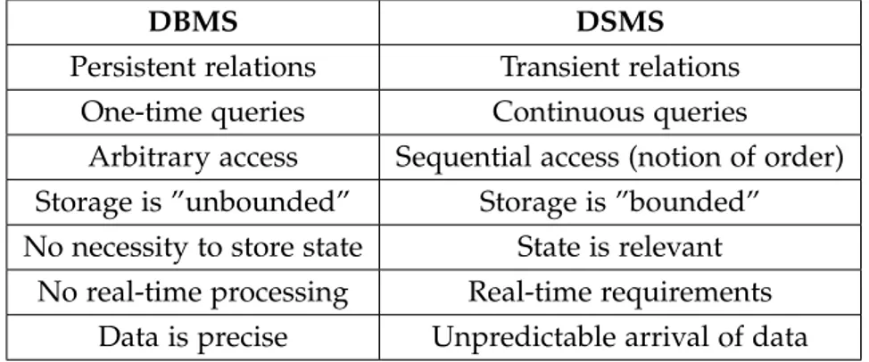
Traditional DBMSs has been developed since the 70’s to answer some of these issues. However the DSMSs have a very distinct architecture as seen in the Figure 1. Just bellow that figure, Table1shows some of the most notable environmental differences that a DBMS and a DSMS have to face with.
In comparison, DBMSs will prevail on situations with persistent relations with one-time queries. There is no relevant importance of time and order, a large storage and possibly more complex queries. On other hand, DSMSs will be more suitable on the previous de-picted situations: transient relations under bounded main memory with notion of time and order and unpredictable arrival of data.
2.2. Real Life Applications of Streaming 5
Figure 1.: Query processing comparison between DBMSs and DSMSs. In DBMSs, the queries are performed on static data and answered immediately. However in DSMSs, queries are made over streams with eventual access to static storage. As queries may run for a very long time, a cache is needed to store the temporary results.
DBMS DSMS
Persistent relations Transient relations One-time queries Continuous queries
Arbitrary access Sequential access (notion of order) Storage is ”unbounded” Storage is ”bounded” No necessity to store state State is relevant
No real-time processing Real-time requirements Data is precise Unpredictable arrival of data
Table 1.: Comparison between a DBMS and a DSMS. In the general scenario, DSMSs behave in a more stochastic environment than DBMSs.
2.2 r e a l l i f e a p p l i c at i o n s o f s t r e a m i n g
The most notable applications of data streams are in the Internet-of-Things field. The City Pulse project, for example, aims to build a framework capable of processing large scale streams of social data in real time in major European cities [Obaid et al.,2012].
The wot.ioTMdata service exchange is a marketplace of web applications that operates on data from connected devices to enable data aggregation, analysis, and an expansive
2.3. Programming Models 6 range of value-added services for enterprise customers [wot.io,2015]. The service has been extended to the SQLstream DSMS to allow to streamline the design and development of IoT applications, and ultimately improve marked adoption.
Using Esper, a Java open source DSMS, a recent study at University of Oslo analyzed streaming data from different medical sensors in real-time to recognize myocardial ischemia with an ECG sensor.
The demand of DSMSs is increasing from sensor networks, so there are frameworks for integration of both technologies [Abadi et al., 2004]. The data streams are widely used on analysis and statistics across many fields. The Gigascope is an example of a stream database for network applications including traffic analysis, intrusion detection and performance monitoring [Cranor et al.,2003].
2.3 p r o g r a m m i n g m o d e l s
The programming model in a streaming platform is one of its most important features, as it determines its possible operations and limitations. At the same time, the model defines the system capabilities and its possible use cases. DSMSs have approached two distinctive programming models to process streaming data: Stream Processing and Batch Processing with both models featuring advantages and disadvantages [Shahrivari,2014].
In Stream Processing also called Native Streaming, the one-at-a-time tuple processing is applied. Data is processed immediately upon arrival, and allows more expressiveness. The reason for this is that the stream its taking control of itself and thus simulates a real continuous flow of data. As tuples are processed upon arrival, the latency in these systems are smaller than on Batch Processing. The existence of state is easier on these systems due to the one-at-a-time tuple processing. On the other hand, these systems are harder to implement, have lower throughput than Batch Processing and fault-tolerance is harder to achieve due to the fact the system has to store and replicate data for every single tuple.
In Batch Processing several tuples are processed at once for a better throughput at a cost of a higher latency. The system’s expressiveness is more reduced compared to Stream Pro-cessing. State management and some operations such joins and aggregations can become harder to implement as the system has to deal with batches of operations. On the other hand fault-tolerance is easier, just by sending batches to every worker node. These systems are applied in scenarios where a huge collection of data is processed at once. There is still the case of Micro-Batching where stream data is processed with much smaller batch sizes [Shahrivari,2014]. The latency is still low and the windowing and state-full computations are easier due to the batch size.
The Stream Processing model was mostly used on the first DSMSs, as it tries to mimic the smoothness of a stream. However the Batch Processing model obtained more importance
2.4. Streaming Query Languages 7 in recent years, due to fact that requirements like scalability and fault-tolerance became predominant in IT. To achieve these requirements, others have to be sacrificed such as the smoothness seen in Stream Processing. Nonetheless is important to note that we can build a Batch Processing system on top of a Stream Processing. However the reverse is more difficult to accomplish when dealing with time.
On meantime, processing high velocity data has brought to two major processing use cases: Distributed Stream Processing (DSP) also called Event Stream Processing (ESP) and Com-plex Event Processing (CEP) [Luckham, 2006]. DSP/ESP is a stateless and straight way of processing incoming data using continuous queries. Data streams are transformed through query operators (joins, aggregations, filters) according to a topology or sequence of instruc-tions. Only the final state is persisted for later analysis. ESP tends handle high volume in real time with a scalable, highly available and fault tolerant architecture. Typical use case scenarios are analysis on-the-fly like in IoT. On other hand CEP, is stateful and batched processing model where state maintenance is always present, hence is better suited for transactional environments. CEP engines try to optimize discrete events in streams while using defined topologies. The state management becomes complex in these systems due to higher requirements in transactional environments. The output can be either persisted or feed to another system. Some examples of CEP are stock exchanges for quick invest-ments, detecting crucial clinic changes from vital monitoring, and accessing political vote intentions.
This report will focus on DSP/ESP for their lower requirements compared to CEP. Build-ing transactional environments for CEP, brBuild-ings extra requirements which is out of scope for this report. At the same time DSP/ESP have better applicability for IoT, but many CEP applications can be rebuild with DSP/ESP [Chakravarthy and Jiang,2009].
It is also important to note that not all DSMSs are built over databases. As an example, messages queues are also often used to implement a streaming engine. Using different models, will result in different approaches to streaming with respective advantages and limitations compared to others.
2.4 s t r e a m i n g q u e r y l a n g ua g e s
Initially defining a SQL query over a stream could be approached on a simple way, just by replacing relations with streams. However when queries get complex with joining, aggre-gation and mixing relations with streams, it becomes necessary to extend the language for separation of concerns. Unlike the SQL standard in DBMSs, there is no standard for the query languages used on the DSMSs. For this reason, query languages vary considerably from system to system [Jain et al.,2008].
2.5. Windows 8 To accomplish the task of creating a specific query language for streams, a new set of models and algorithms should be implemented as well. For this reason, most DSMSs expose these models and algorithms on their query languages.
To process data incrementally, the windows concept became an essential component of most DSMSs. Windows are buffers of data able to store streams’ tuples in memory. Win-dows operate according to fixed parameters such as the size and bounds of the window, being these parameters updated after each query call [Ghanem et al., 2007]. Therefore in most DSMSs Query Languages, windows are used implicitly to process data incrementally. The windows concept will be explained in detail in Section2.5.
The query operators must also be revised to accommodate both streams and persistent relations [Law et al.,2004]. Therefore different types of operators have been built to address several possible scenarios. The overview of query operators is given on Section2.6.
SensorBee is an open source stream processing engine dedicated to IoT. SensorBee query language was derived from CQL, the language from STREAM, one of the first DSMSs declarative languages integrating streams with persistent relations [Arasu et al.,2006]. Now taking a sample query of a shopping website using streams:
SELECT P.price * (1 + P.tax) AS TotalPrice FROM Orders[RANGE 5 TUPLES] AS O, Products AS P WHERE O.ProductID = P.ProductID;
”Products” is a table listing the information of the products with respective prices and taxes. ”Orders” is a stream of incoming orders in the shop. [RANGE 5 TUPLES] specifies a 5 element sliding window, which means the query will be executed whenever 5 orders are made in the website.
However the main question is how we should interpret this query: Can a product’s price change between query calls? How we know if we are returning a relation or a stream? If the current transaction rollbacks, should we put the last window orders back on the stream? In general, the streaming concept introduces several implementation issues: The aggregations on streams should be based on the current window, or the whole stream? It’s feasible to join streams? How to trigger a query which uses two streams with different windowing parameters? Can we reuse the same stream tuples on multiple queries? All these questions must be answered by the DSMSs themselves at their implementation.
2.5 w i n d o w s
The desirable feature in DSMSs is to approximate stream processing likewise persistent relations. A common approach is to partition the stream in windows. Each window is comprised by a finite bag of tuples and processed sequentially. Also a window has an
2.5. Windows 9 implicit notion of order, which means the tuples belonging to it are ordered according to a specific attribute. The number of valid elements in an window determines its type, and varies through the window dimension unit, edge shift and progression step.
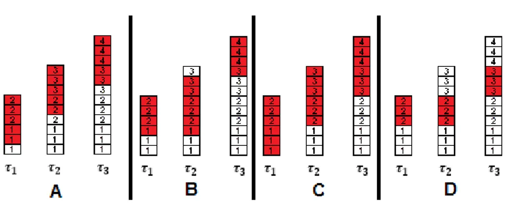
The dimension of a window can be measured in either two ways: a time-based window through a τ units of time, or a tuple-based window meaning x first elements in the window are valid for the query at the time, likewise a FIFO queue. For both models, the inclusion of a timestamp in tuples is important for ordering in the queue. However some systems have introduced windows with other ordering criteria. Aurora added value-based windows, in which the windowing attribute is any other field [Abadi et al.,2003]. Other systems added predicate-windows where the window is filled until when a tuple fails a pre-defined condition [Ghanem,2006]. At Figure2, window C is a sliding time-based window with temporal extent (number of timestamps at the window) ω=2 and progression step δ=1. Also window A is a count-based sliding window (a variant where the window always take the last n tuples, in this case 5).
Meanwhile the edge shift specifies the movement from the bounds of the streams. The shift can be either fixed or moving along with the stream. In sliding windows, both bounds move along with the data arrival. Some languages use the SLIDE parameter for this specification [Kajic,2010] (e.g. [RANGE 10 SECONDS SLIDE 5 SECONDS] Once 10 seconds have passed, the window moves forward by 5 seconds). In landmark windows only one of the bounds moves, meanwhile on the tumbling windows there is an arbitrary progression step of both bounds. At Figure2, window B shows a landmark window with the lower bound fixed at τ, resetting after every 6 new tuples. Window D shows a tumbling window of temporal extent ω = 1 and progression step δ=2.
Finally the progression step defines the periodicity of windows movements. Like the mea-surement unit, the step can either be time or tuple based (move every 10 seconds or 15 new tuples). In this specification, tuples overlap in more than one window. Nonetheless in tumbling windows, there is a moment where all tuples in a window become invalid at the same time. It is important to note that distinct window specifications will be applicable to different specifications. For an aggregation operator, a tumbling window will be more advantageous; while for a join, a sliding window is preferable [Patroumpas and Sellis,2006].
2.6. Streaming Operators and Continuous Queries 10
Figure 2.: Comparison of some windows implementations (A, B, C and D) with different edges shift and progression steps trough time instants τ1, τ2 and τ3. New tuples arrivals are placed
at the top. The number in the tuples represent their current timestamp. The window at instant τxis represented in red.
2.6 s t r e a m i n g o p e r at o r s a n d c o n t i n u o u s q u e r i e s
Due to explicit constraints on streaming data, a revised set of operations for the query lan-guage is beneficial to DSMSs [Law et al.,2004]. In many applications, statically stored data is used with the streams to produce results. An example scenario is when historical data is updated with new incoming data. Therefore there is a necessity to join data from multiple streams and static data simultaneously. For this reason is necessary to re-implement the existing operators into Stream-to-Relation, Relation-to-Stream and Stream-to-Stream operators. Most DSMSs support Stream-to-Relation and Relation-to-Stream operators. Stream-to-Stream operators are more complicated to implement. For example in stream joining, the general approach for is to interpolate one of the streams as a persistent relation through sampling, turning to the situation of joining a stream with a persistent relation [Das et al.,2003].
In DBMSs ad hoc queries run through a set of operators which wait for all input before producing results. Due to continue flow of data in DSMSs, this implementation isn’t feasi-ble. To go over this, queries in DSMSs perform incrementally using continuous queries and reviewing a new set of operators.
For this reason, continuous queries have high importance in DSMSs, as it is not feasible to store the entire stream and then process it like in DBMSs [Babu and Widom, 2001]. Depending on external conditions, query statements might wait very long between arrivals of data in order to produce results. Varying from the operator’s complexity the continuous queries might be harder to implement. For example, aggregation queries might require grouping changes with small computations, but join queries might produce an unbounded answer which is not feasible. To tackle this, blocking query operators were introduced so the queries are processed periodically instead at whole once.
2.7. Time and Order 11 At the same time, non-blocking query operators produce results sporadically, or on arrival of some tuples as it happens on some aggregation operators.1
These operators are more suitable to continuous queries, however not all queries can be expressed with these type of operators [Law et al.,2004].
Another important distinction in DSMSs are stateless operators and stateful operators. The last ones (e.g. joins) require storing the intermediate state of their operations as the streams are unbounded. An immediate question is where and how to store the state between continuous queries calls while being fault-tolerant and scalable [Fernandez et al.,2013].
Now is important to note that this revision will vary considerably between Stream process-ing and Batch processprocess-ing systems. The former ones prevail over stateful and blockprocess-ing query operators to update each continuous query for each incoming tuple, while the latter ones prevail over stateless and non-blocking query operators for more efficiency.
Taking again SensorBee as an example, the following query outputs the join between a stream and a standard table in the database. It is expected to count the number of sells of all Amsterdam’s merchants in the last 60 seconds. The [RANGE 60 SECONDS] is a Stream-to-Relation operator, responsible to convert the current window to a relation in each continuous query call. The ISTREAM is a Relation-to-Stream operator which creates a stream that only emits tuples present in the current window, but weren’t so in the previous one. Therefore will be only outputted notifications of sells updates in the last 60 seconds.2
SELECT ISTREAM M.name, COUNT(*) AS total_count FROM Sells [RANGE 60 SECONDS] AS S, Merchants AS M
WHERE M.merchantID = S.merchantID AND M.address LIKE ’%Amsterdam%’ GROUP BY M.name;
2.7 t i m e a n d o r d e r 2.7.1 Timestamps
In data streams, the notion of time is very important for ordering tuples in time based windows. The first question is how the values are timestamped. The general solution is to add an extra field to the tuples. The next question is to consider a logical or a physical way of timestamping. In the former each tuple is enumerated using a counter (e.g. a Lamport timestamp) but it serves just for ordering. In the later, the time information from the system is used (e.g. an UNIX timestamp) but systems differ in their timestamp interpretations. In many systems, internal timestamps are used whenever a new element arrives in the system
1 The aggregations can either be blocking or non-blocking depending if the data is sorted or not. More informa-tion on:http://sqlsunday.com/2014/06/15/blocking-aggregate-operators/
2 More information about these operators can be found at SensorBee’s documentation: http://docs.sensorbee. io/en/latest/bql.html#relation-to-stream-operators
2.7. Time and Order 12 [Bai et al.,2006]. This guarantees that tuples are ordered by arrival time, and while they are pipelined through the system. In contrast, external timestamps are created by the external sources as an attribute, then ordered inside the system [Bai et al.,2006].
Some systems order the tuples for the same timestamp by arrival order. This is necessary to avoid semantic inconsistencies in some queries that can be provided from windows. At Figure 2, in C window, tuples of the same timestamp are present at same window. As an example, an unordered sequence could provide wrong results for the median value of a window.
Another relevant question is how to correctly assign timestamps after the results of n-ary operators. For aggregations, the result of a windowed minimum or maximum query could use the timestamp of the maximal or minimal tuple. In a count, sum or average the timestamp of the latest tuple could be kept. In a join a general solution is to timestamp the value of the tuple of the first table (in FROM clause), which can be used for external and internal timestamping models. A more generic attempt is to use the median value of the window.
2.7.2 Order
Generally speaking, many systems rely on the order of their elements for correctness. Also some operators become more efficient with the ordering of the input (e.g. usage of indexes). In DSMSs, ordering is easier due to sequential arrival of data. However this can be hard to achieve in systems with external timestamps from multiple sources. Since then, two solutions have been proposed for possible disordering problems.
The first solution is to tolerate disorder in stream’s limits. In the Aurora system, tuples do not need to be ordered by timestamp [Abadi et al., 2003]. This imposition allows to split operators in order-agnostic and order-sensitive operators. The first group does not rely on order (filter, map and union) and therefore are executed efficiently. The second group (bsort, aggregate and join) have parameters on how unordered tuples should be handled. All other unordered tuples will be discarded through load shedding [Abadi et al.,2003].
The second solution is to indicate the order of tuples and reorder them whenever is necessary. Although the use of internal timestamps provides order, systems semantics with multiple sources require external timestamps. In some systems such as Gigascope, Heartbeat tuples are sent with the stream including a timestamp [Johnson et al.,2005]. These marks indicate that all following tuples require to have a greater timestamp than the mark itself. Heartbeats can be created by the sources or by the system itself.
2.8. Query Optimizations 13 2.8 q u e r y o p t i m i z at i o n s
The internal query execution is very similar to the one we find in DBMS, however the query optimization becomes very different in DSMS. In query optimization in DBMSs, we calcu-late several possible plans for a query, then we choose the least costly one using tables’ car-dinalities. This process differs in DSMSs because the cardinality calculation is problematic in a streaming environment. Also DBMSs storage statistics of data to help in optimization, but in DSMSs since the data of streams is unknown in advance, there are no such statistics. However it is possible to examine a data stream for a certain time to obtain a summary of the stream. Earlier DSMSs typically applied a plan migration strategy to replace a query plan with a new one at execution through time when the summary was obtained [Zhu et al., 2004].
The first common optimization technique is the Rate-based optimization, where rates of streams are taken in consideration in the query evaluation tree during the optimization process [Viglas and Naughton,2002]. Instead of choosing the least costly plan, it is possible to decide for the plan with the highest tuple output rate. In advance it is required to derive expressions for the rate of each operator. As an example, we have a very fast selection operation on 100 tuples/second and a slower selection operation on 10 tuples/second. Both operations have the same selectivity of 0.1 tuples/s and can be commuted. Supposing we have a stream input of 200 tuples/s, if the slower operation happens first, by the first operator we have a throughput of 1 tuple/s by the first operator, then 0.1 tuples/s after the second. However if the faster operation occurs first we have a throughput of 10 tuples/s by the first operator, then 1 tuple/s after the second (about 10 times faster).
Often data streams obtain abnormal high inputs of data than usual producing longer queues of unprocessed elements. Operator Scheduling deals with tuple arrival rate and the operator path to answer against these situations [Babcock et al.,2004]. If the arrival rate of the tuples is uniform and lower than the system capacity, then there will be no problems in terms of scheduling. Whenever a tuples arrives at the system, we schedule it through all the operators in its operator path. In conclusion we refer this strategy as FIFO (First In, First Out), which is common through queueing systems. However we should note that unifor-mity in arrival is just a possible scenario, and hence we need more sophisticated scheduling strategies guaranteeing that the queue sizes do not exceed the memory threshold.
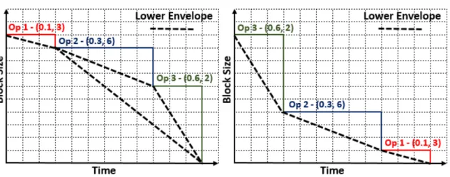
The Chain Scheduling Algorithm is used in DSMSs to manage queues and productivity of operators [Qian and Lu, 2010]. Suppose that each operator has a pair of selectivity and time to process(σ, τ). Later is possible to order them based on these two values. Operators with lesser time to process and more selectivity will have higher priority scheduling them first. A chart as seen on Figure3is built based on these pairs using three random operators
2.8. Query Optimizations 14 with different times to process and selectiveness. The input is buffered between operators as shown in the Greedy algorithm.
Figure 3.: Arrangements for operators with selectivity and time to process(σ, τ)in Chain scheduling
resulting in distinct lower envelopes.
Chain Scheduling results in a lower envelope which represents the best case of the Greedy algorithm. A proper ordering of the operators might result in a smaller lower envelope, and therefore smaller queues and less memory requirements. An lower envelope will be better if it has a lower total area. Chain Scheduling helps to minimize memory usage, but CPU may be the bottleneck. Taking time in consideration, approximate answers are often more useful than delayed exact answers. So whenever an input stream rate exceeds the system’s capacity, a stream manager can drop tuples. Now the goal is to minimize inaccuracy in answers while keeping up with the data.
The main concern is how often we should drop tuples, and thus becomes a challenging problem for the quality of results. The load shedding addresses this issue. A study calculated an optimal formula to estimate the error rate on sliding window aggregate queries with sub-queries on STREAM project [Mayur et al.,2003]. The algorithm has two steps: accumulate sampling rates for the queries (average and variance), then calculate a probability p for every tuple that will be used to discard it or not according to the equation. When there is only one operator in the query, it’s straightforward, however, when some operators are shared by multiple queries, the situation becomes more complicated, since distinct queries require higher or lower sampling of tuples to produce the same maximum relative error estimate. Also there is a compromise of using load shedders earlier or late on a query plan (efficiency vs. accuracy) [Mayur et al.,2003].
Instead of optimizing the processing engine, another possible approach is to process less data for better latency and memory, thus achieving faster response in queries. Synopsis structures are commonly used to compress incoming data to achieve these requirements
2.9. Streaming Engines Outline 15 [Gibbons and Matias, 1999]. These structures include making sampling on windows [Al-Kateb et al.,2007]; creating a compact synopsis of the data that has been observed through sketches [Matusevych et al.,2012]; creating a history of observations with histograms [Guha et al., 2006]; making hierarchical decomposition of incoming data with wavelets [Garo-falakis,2009].
2.9 s t r e a m i n g e n g i n e s o u t l i n e
Having discussed a variety of challenges addressed and features offered by different DSMS, this section describes a set of representative systems and focuses on how they offer various design and implementation trade-offs.
The growth of demand for streaming data and distribute system behavior, brought more requirements for these systems. The message delivery guarantees is an imposing rule indicat-ing that output and input tuples must be delivered eventually. At the same time, failures can happen anywhere: network down, disk failures, nodes going down for maintenance might compromise the system. Fault tolerance rules how well the system reacts to failures and recovers from them. As discussed on Section2.6, state management has high importance of research in stream data. How the state is kept and updated is another important point of implementation in these systems.
Meanwhile the ”big” companies have introduced streaming engines in their products. MillWheel, developed by Google [Akidau et al., 2013], provides a fault tolerant directed computed graph in which the system manages persistent state and the continuous flow of records with low-latency. Trill, developed by Microsoft [Badrish Chandramouli,2015], uses a tempo-relational model to handle arriving tuples with immediate results, while providing high performance. FlumeJava, also developed by Google [Chambers et al.,2010], uses the MapReduce programming model to handle high performing parallel pipelines that can be used on streaming data.
2.9.1 Apache Storm
Apache Storm is a distributed platform for Java focused on streaming data using the Stream Processing programming model with absence of windows.3
. It has become an Apache Project in 2014 after being acquired by Twitter [Toshniwal et al.,2014].
Storm provides nodes to manipulate streaming tuples using three abstractions: spouts, bolts, and topologies. The spouts are the streams sources, where the user specifies how streams are generated. Bolts are responsible for the business logic of the streams. This logic includes filters, joins, aggregations and database interactions. Spouts and bolts are
2.9. Streaming Engines Outline 16 ganized into networks known as topologies. Topologies are Directed Acyclic Graphs (DAGs) with each node representing a bolt or a spout. Edges are represented by subscriptions to subsequent bolts, hence the topology is seen as the computation process of streams. After deployment, the topologies will run indefinitely until killed.
Storm’s topologies are parallel by default, running in scalable and fault-tolerant clusters. The clusters are comprised of a master node daemon called ”Nimbus”, whose task is to distribute code instructions around the cluster, assign tasks and monitor failures. The workers run in a daemon called ”Supervisor” who listens to tasks provided by Nimbus, for its own topology. A Zookeeper cluster is used to coordinate the communication between Nimbus and Supervisors [Toshniwal et al.,2014].
In recent years, Apache Storm suffered several scaling problems, and therefore the Twitter team developed a new streaming engine to face these issues: Apache Heron [Kulkarni et al., 2015].4 Heron continuously examines the data in motion and computes analytics in real-time with better debugging and efficiency. It was open-sourced in May 2016.
2.9.2 Apache Spark Streaming
Apache Spark is a cluster computing framework influenced by Apache Hadoop’s MapRe-duce programming model, having started in 2014.5
Spark is notable for processing data in batches in its whole framework, answering today’s scaling requirements. For this reason it has become one of the most active open source big data projects today [Harris,2015].
Apache Spark contains several APIs within its framework for batched applications. These APIs include Spark SQL for data persistence; GraphX, a distributed graph processing li-brary: MLlib (Machine Learning Library), a distributed machine learning library; and Spark Streaming, a library for stream data processing. Spark Streaming is a scalable, high throughput and fault-tolerant data stream processing system. While Hadoop’s MapReduce is considered a case of Batch Processing [Shahrivari, 2014], Spark Streaming uses the Micro-Batch Processing model operating in smaller batch sizes compared to Hadoop.
The Spark’s API is centered around Resilient Distributed Datasets (RDDs), a data struc-ture of read-only data distributed over a cluster of machines on a DAG while fault-tolerant [Zaharia et al., 2010]. For this reason Spark internally slices data into batches to be dis-tributed, hence its programming model. As a consequence, the results are also produced in batches.
Spark Streaming extends Spark Core’s to perform streaming analytics. It takes data in mini-batches and operate RDD transformations on those batches at cost of higher latencies. The data can be provided through related open source libraries (e.g Apache Kafka) or barely
4 Website:https://twitter.github.io/heron/GitHub repository:https://github.com/twitter/heron 5 Website:https://spark.apache.org/GitHub repository:https://github.com/apache/spark
2.9. Streaming Engines Outline 17 with a TCP connection. The streaming operators are provided through a functional interface with operations such as map, reduce and join [Zaharia et al.,2010]. These operations take RDDs as input and output RDDs as well for integration with other Spark APIs.
2.9.3 PipelineDB
PipelineDB is a stream extension of PostgreSQL open-sourced in 2015. This project will be more comparable to MonetDB’s approach due to perform streaming with databases.6
The continuous queries concept is present through continuous views. The continuous views are materialized sets of results which are updated through time using time based windows. As soon as a tuple of a stream is read by the view, it will be processed and discarded, hence applying the stream processing model. This implementation gives predominance on the continuous views over streams. As a consequence if more than one stream is featured in a single continuous view, the windowing method applied will be the same for all the streams, hence this dominance.
It is also possible to integrate incoming streams with static data through continuous joins. Stream to table joins are performed whenever a tuple arrives, joining it with matching rows and updating the continuous view immediately. Note that if other matching rows in the persistent relation are inserted after the tuple arrival, the continuous view will not be updated as expected. The same happens whenever rows are updated or deleted.
To achieve fault-tolerance, PipelineDB supports streaming replication, using the passive replication approach. PipelineDB also has support for message queues through an integra-tion with Apache Kafka.
However there are no tuple based windows, stream-to-stream joins are not supported, and due to usage of continuous views there is no native support to output stream data in physical devices. Nonetheless, this can be achieved by continuous transforms, which call user defined procedures whenever continuous views are updated, for producing output streams.
In the following example, the page_views stream collects URLs requests storing clients cookies and the latency of the request for benchmarking. Later the page_stats continuous view aggregates data from page_views in the last 10 minutes using a sliding window. For each URL it calculates the views count, unique visits using cookies and the 90th value percentile of the latency.
CREATE STREAM page_views (url text, cookie text, latency integer); INSERT INTO page_views (text, cookie, latency) VALUES ( ... );
CREATE CONTINUOUS VIEW page_stats WITH (max_age = ’10 minutes’) AS
2.9. Streaming Engines Outline 18 SELECT
url::text,
count(*) AS total_count,
count(DISTINCT cookie::text) AS uniques,
percentile_cont(0.9) WITHIN GROUP (ORDER BY latency::integer) AS p90_latency FROM page_views GROUP BY url;
2.9.4 DataCell
DataCell was a DSMS extension of MonetDB, developed by Dr. Erietta Liarou between 2006 and 2012 [Liarou,2013]. DataCell was positioned in the Back-End layer of MonetDB (Section 3.3), and was able to process continuous queries. After the creation of a continuous query, its optimizer generated the respective execution plan and handed it over to a scheduler who would be responsible to control the plan’s life-cycle [Liarou et al., 2013]. To handle input and output, DataCell enclosed a set of receptors and emitters, which took advantage of MonetDB’s column-based architecture to store data [Liarou et al.,2013].
3
M O N E T D B O V E R V I E W3.1 c o l u m n-wise storage
MonetDB is a RDBMS with a column-wise storage, opposed the traditional RDBMSs which use a row-wise storage. MonetDB was initially designed for Business Intelligence research often comprised by large data warehouses. These applications integrate large databases where an efficient access of data is required. The same scenario happens in e-science field where large bulks of data are inserted simultaneously for research purposes [Idreos et al., 2007].
Through the years, MonetDB has researched new ways to build these databases more efficiently and scalable, while taking advantage of column-wise storage.
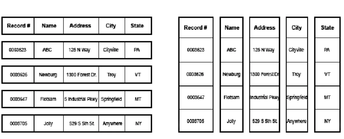
Figure 4.: Internal representation of row and columnar-wise storage. The columnar storage provides better cache usage for a single column access, as well it creates more opportunities to compress data. Image taken from: http://arxtecture.com/wp-content/uploads/2014/ 01/row-store-v-column-store.gif
3.2. Internal Representation 20 3.2 i n t e r na l r e p r e s e n tat i o n
The storage model in MonetDB is also different from traditional DBMS due to its columnar store. MonetDB handles relations tuples in Binary Association Tables (BATs) [Idreos et al., 2012], meaning for a relation with k attributes, there will be k distinct BATs for that relation. A single BAT contains data corresponding to the data type of a column. A table is then represented by a collection of BATs. After loading BATs into memory, they are accessed as an ordinary C-array using Object Identifiers OIDs.1
It is important to note that OIDs are never serialized, just calculated on execution time depending on the data type of the column, allowing efficient operations like COUNT aggregations with O(1)cost. For variable length data types such as strings and BLOBs, MonetDB builds a heap of these values. BATs of the same value, are loaded into the same heap entry allowing further compression.
MonetDB uses the operating system’s memory mapped files functionality to load persis-tent data, meaning that the binary representation in memory and the disk is the same, thus avoiding conversions. In addition to this, MonetDB uses late tuple reconstruction, meaning that all the intermediate query results are stored column-wise [Idreos et al., 2012]. Result-ing relations are built just before sendResult-ing them to the user. This technique allows to exploit CPU caches as well vector-wise operators for a more efficient processing.
On the other hand, column-wise storage might expose performance issues during rela-tions updates. As the relarela-tions tuples are stored across several sources, a write operation across several columns simultaneously can be I/O expensive. To alleviate this, MonetDB uses delta structures kept in memory [H´eman et al.,2010]. For each column there is a inser-tion and a removal delta structure alongside. During a transacinser-tion, instead of writing new changes to the sources immediately, they are written to these structures in memory. After the transaction is committed, the delta structures are merged with the respective columns in the sources.
The BAT representation is manipulated by MonetDB’s kernel through the MonetDB As-sembly Language (MAL). In its core, a relational algebra operator corresponds to a MAL instruction, meaning that each BAT algebra operator translates into a single MAL instruc-tion. The conjunction of MAL statements for a SQL query is called a MAL plan. MAL instructions are evaluated with an operator-at-time schedule, meaning that each operation is evaluated completely before executing the next one. Complex operations are broken into a sequence of BAT operations that each perform on a entire column of values, known as bulk processing [Idreos et al., 2012]. The bulk processing mechanism allows loops without func-tion calls, creating high temporal locality which reduces cache misses. Also these loops are
1 The BAT term was initially used to define an attribute with both a head (OID) and a tail (value). However as of June 2016, heads were removed completely from BATs as they are calculated on execution time. Therefore the term BAT may lead to confusion meaning that there is a binary relation but it is not.
3.3. Query Processing 21 more susceptible to compiler optimizations such as loop pipelining, and CPU out-of-order speculation.
The following example shows the MAL instruction for a selection on a integer column B for values equal to V into the result set R, while showing the respective C equivalent code.2
The result set is a collection of OIDs of selected rows. The value of n in for loop is calculated based on the data type of the column and its size beforehand.
R:bat[:oid] := select(B:bat[:int], V:int);
for (i = j = 0; i < n; i++) { if (B[i] == V) { R[j++] = i; } } 3.3 q u e r y p r o c e s s i n g
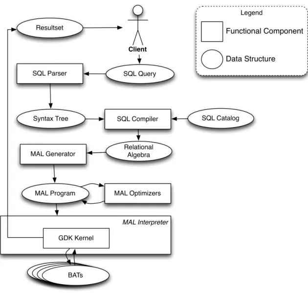
MonetDB’s query processing scheme is performed through three software layers: Front-End, Back-End and Kernel [Idreos et al.,2007].
The Front-End layer is responsible to parse SQL queries and convert them to MAL execu-tion plans. The processing scheme begins with the SQL Parser translating an input query into a specific Syntax Tree. On the next phase, the SQL Compiler has responsibility to pro-cess the generated Syntax Tree and translate it into a logical plan, then to the respective MAL execution plan with some optimizations. These optimizations are performed at exe-cution time and aim to reduce the size of input to be handled on the Back-End. The applied optimizations vary from the properties of the columns such as the data type, ordering or existence of an index.
Further optimizations are performed at the Back-End layer through the MAL Generator. The MAL Optimizer is a sequence of modules to manipulate a given MAL Program into a more efficient one. Unlike in the Front-End, the optimization in Back-End is inspired by programming language optimization instead of SQL optimization [Idreos et al.,2007]. For instance there is a set of optimizers for parallel query plan generation [Milena Ivanova and Groffen, 2012], which is made possible with column-wise storage. The mitosis optimizer splits the relation attributes into smaller chunks based on the number of available CPU cores. The mergetable optimizer merges the partial query results after all sub-queries have performed. It is important to note that some instructions cannot be executed in parallel, so they are not optimized further in order to warranty the correctness of the results. These
2 Adapted from MonetDB official website: https://www.monetdb.org/Documentation/Manuals/MonetDB/ Architecture/ExecutionModel
3.3. Query Processing 22 instructions are called blocking instructions.3
The mergetable waits for all parallel instructions to finish, packing the result columns together, before calling a blocking instruction.
The Kernel layer also called Goblin Database Kernel (GDK), is responsible to perform CRUD operations on BATs, as well handing over a highly optimized library of the binary relational operators. As a consequence of bulk processing, each relational operator has access to the input’s properties at execution time, therefore they judge the implementation algorithm also at execution time. As an example, a join operator decides at runtime to execute a merge-join if the correspondent attributes are sorted, or a hash-join if that condition does not happen.
Figure5shows all MonetDB’s functional components and the generated data structures during the processing of a SQL query.
Figure 5.: MonetDB’s components and relations during the execution of a SQL query.
4
A I O TA P L AT F O R M4.1 d e s i g n c o n s i d e r at i o n s
The Internet-of-Things growth, has led to increasing demands in streaming processing, hence building software solutions capable to answer the demand is notorious. At the same time, research in MonetDB focused on large databases through the years with focus on performance, which can be exploited to build a reliable streaming engine.
The proposed platform is called AIoTA (Amsterdam Internet-of-Things Application), to accommodate the IoT interest raise in Amsterdam city in the last years, with special atten-tion to the recently proposed Amsterdam IoT network [de Vries, 2015]. The following list contains the main objectives for this platform:
1. Offer an interface for IoT devices, with low requirements and usability. 2. Add a flexible streaming extension to MonetDB’s engine.
3. Assemble a topology vector-like to take advantage of MonetDB’s columnar architec-ture.
4. Build an architecture easy to scale horizontally and vertically later on.
5. Provide an easy interface for monitoring and analyze the output, with a notification API.
Extending MonetDB with a continuous query processing capability is only one thing we need to do in the bigger picture. Next to that we need to build a full stack platform capable to collect, process and deliver streaming data in a transparent way to the IoT world. During this project a platform has been developed aiming to satisfy the previous stated requirements.
4.2. AIoTA Architecture Overview 24 4.2 a i o ta a r c h i t e c t u r e ov e r v i e w
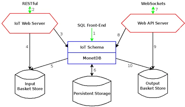
Figure 6.: AIoTA’s proposed platform, components and relations.
The full AIoTA platform is depicted at Figure 6. AIoTA’s topology exposes two web servers for IoT devices: IoT Web Server and Web API Server (red boxes), as well the reg-ular SQL Front-End whenever is desirable to make a direct connection with MonetDB’s engine. Meanwhile MonetDB’s kernel code (blue box) is extended for AIoTA.
In the whole AIoTA’s topology, is noticeable the usage of baskets as intermediate storage. Baskets are sets of binary representations of BATs. Since MonetDB’s columns are stored using this representation, providing data immediately on the same representation allows a better performance while importing and exporting it using MonetDB’s binary import feature.1
Meanwhile, both web servers and the MonetDB instance run on distinct processes, hence the baskets act as the way of inter-process communication.
In the left side of Figure6, (arrows 2, 3, 4 and 5) show the flow of IoT Web Server. This web server is responsible to collect and validate inputs from IoT sensor devices and translate them into streams’ input using MonetDB’s internal representation in the input baskets.
The generated baskets by the IoT Web Server are collected by the MonetDB’s engine for processing. This engine includes a new streaming extension under the ”iot” database schema (1). In this schema, a scheduler whichis responsible to manage the existing
con-1 More information about the binary import here: https://www.monetdb.org/Documentation/Cookbooks/ SQLrecipes/BinaryBulkLoad
4.3. AIoTA Workflow 25 tinuous queries. The streaming data can also be assimilated with other database objects (e.g. tables, functions, procedures) on persistent storage (6).
The MonetDB’s engine generates output data in the form of baskets for the Web API Server, with its flow shown in the right side of Figure 6(arrows 7, 8, 9 and 10). This web server is responsible to translate the output the baskets to IoT monitoring devices.
4.3 a i o ta w o r k f l o w
The IoT Web Server provides a RESTful interface, listening to HTTP JSON requests (2). The RESTful systems provide simple interfaces, approachable by IoT devices [Gruetter, 2012]. This server connects with the streaming extension (3) to create and delete streams and inserting data over its lifetime inside the Input Basket Store (4). The development of IoT Web Server is detailed in Chapter5.
Incoming data stored inside the Input Basket Store, is processed by the streaming extension (5) inside MonetDB. It is important to note that the baskets contains volatile data, so once they have been consumed by the continuous query engine, they are deleted immediately as a recurrent behavior of DSMSs (Section 2.1). Continuous query results are stored on Output Basket Store by the new streaming engine on MonetDB. (10), later consumed by the Web API Server (9). Eventually the query results can be stored in regular MonetDB tables as persistent relations (6) instead in the output baskets. The development of the new streaming engine under the ”iot” schema is detailed in Chapter6.
The Web API Server looks up for existing streams in the streaming context (8). This server reads and converts data from Output Basket Store, while exposing it to a Web API using the WebSockets protocol (7). With WebSockets, it is possible to manage real time monitoring of events in IoT using a full-duplex connection. Therefore the web client can subscribe to be notified immediately whenever new output baskets are created. The development of Web API Server is detailed in Chapter7.
This platform handles streaming data using a Batch Processing model (Section2.3), taking advantage of MonetDB’s vectorized architecture for processing in batches. At the same time, many IoT networks behave likewise Wireless sensor networks (WSNs) [Alcaraz et al., 2010]. WSNs are comprised by distributed autonomous sensors for monitoring, where data is sent cooperatively between them to a main collector for processing. This approach results in sending data in batches, hence is advantageous for AIoTA. AIoTA performs under a Distributed Stream Processing model (Section2.3) as it provides more flexibility and lower requirements compared to CEP during the internship time.
5
I O T W E B S E R V E R I M P L E M E N TAT I O NThe IoT Web Server aims at an easy API for IoT, so it hides the underlying streaming and database layers for IoT sensors. The IoT Web Server is written in Python using the Flask-RESTful framework, a popular Python library for Flask-RESTful web servers.1
The IoT Web Server is capable of creating and deleting streams on AIoTA using a RESTful API. After a stream is created, it is possible to make batch inserts into it. Both stream creation and stream insertion are validated using an official JSON Schema.2
In the current implementation, a batch of tuples will be inserted, if only all the tuples are valid. This approach will force further correction on a batch, meaning that a batch is correct if and only if all its tuples are also correct, as in transaction processing. As discussed in Section 2.7, the server adds an implicit timestamp column to perceive when the tuple was inserted. Inserted tuples are later imported to the corresponding streams in the streaming engine and consumed by the respective continuous queries.
5.1 r e s t f u l s y s t e m s
The REpresentational State Transfer (REST) is an architectural style with a specific set of conventions and components to build web applications, where the focus is to specify the components roles, and interactions instead of concentrating on implementation details. The term was introduced in 2000 by Roy Fielding [Fielding,2000].
Systems that employ the REST style are called RESTful. On RESTful systems such as the IoT Web Server, clients approach the web server using the HTTP protocol, and use the HTTP methods GET, POST, PUT and DELETE to discriminate their requests. RESTful systems expose their features using web resources identified by Uniform Resource Identifiers (URIs). For example, in IoT Web Server, /stream/measures/temperature is a URI to identify the stream ”temperature” in the schema ”measures”. To achieve the desired properties, REST defines several principles that should be followed by the RESTful systems:
1 Flask-RESTful at PyPI:https://pypi.python.org/pypi/Flask-RESTful
2 Over the JSON Schema: https://spacetelescope.github.io/understanding-json-schema/ The version used is from the latest draft (4).