Universidade do Minho
Escola de Engenharia
Departamento de Inform ´atica
Master in Informatics Engineering
Jo ˜ao Tiago Ara ´ujo da Silva
Molecular dynamics simulation in hybrid systems
Master Dissertation
Supervised by: Jo ˜ao Lu´ıs Ferreira Sobral
Ant ´onio Joaquim Andr ´e Esteves
A G R A D E C I M E N T O S
Antes de mais, gostaria de agradecer ao meu orientador Professor Doutor Jo˜ao Lu´ıs Sobral e ao meu co-orientador Professor Doutor Ant´onio Joaquim Andr´e Esteves pela disponibilidade que sempre demonstraram na resoluc¸˜ao de problemas e duvidas surgidas no desenvolvimento desta tese e pela realizac¸˜ao de reuni˜oes semanais. Tamb´em gostaria de agradecer ao aluno de doutoramento Bruno Silvestre Medeiros pela disponibilidade demonstrada e pelos seus conselhos e sugest˜oes. Finalmente gostaria de agradecer `a minha fam´ılia o apoio incondicional e pelo incentivo que me deram a todos o n´ıveis.
A B S T R A C T
The molecular dynamics simulation is a topic fairly investigated because it solves countless prob-lems of physics, chemistry, or biology. From the computer engineering point of view it is an interesting case study because it is a computationally complex problem. The complexity arises when there are a high number of particles, thereby resulting in a high number of iterations to compute on each iteration. Presently there are systems with millions of particles that need to be simulated in the shortest time possible. This led to the development of molecular dynamics packages that attempt to use all the resources available to improve the execution of simulations. The main goal of this thesis is to run efficiently molecular dynamics simulations on hybrid sys-tems. Instead of starting a molecular dynamics implementation from scratch, it was used the MOIL package. Then it was developed an implementation based on MOIL with optimizations that allow the code to be automatically vectorized by the compiler. These optimizations focused on the calculation of forces and the data structures. New data structures were introduced to de-compose the simulation domain into cells. The vectorization was used both in sequential and parallel implementations. In both cases, vectorization allowed a higher performance when used with cells. In order to achieve the best possible performance, the optimized code has been par-allelized using different strategies, including shared memory, distributed memory, and a hybrid solution. In the execution of the parallel code several combinations of processes and threads were tested. Among all the developed versions, the one that achieved the best performance was the hybrid version. All implementations were compared to Gromacs, the reference in terms of performance of the molecular dynamics simulation.
R E S U M O
A simulac¸˜ao de dinˆamica molecular ´e um tema bastante investigado porque permite resolver in´umeros problemas da f´ısica, qu´ımica, ou biologia. Do ponto de vista da engenharia inform´atica ´e um caso de estudo interessante por ser um problema computacionalmente complexo. A com-plexidade surge quando se utiliza um elevado n´umero de part´ıculas, necessitando assim de se calcular um grande n´umero de interac¸˜oes em cada iterac¸˜ao. Atualmente h´a sistemas com milh˜oes de part´ıculas que se pretende que sejam simulados no menor tempo poss´ıvel. Este facto levou ao desenvolvimento de ferramentas de dinˆamica molecular que procuram utilizar todos os recursos dispon´ıveis para melhorar a execuc¸˜ao das simulac¸˜oes.
O principal objetivo desta tese ´e executar eficientemente simulac¸˜oes de dinˆamica molecular em sistemas h´ıbridos. Em vez implementar a simulac¸˜ao de dinˆamica molecular desde o in´ıcio, foi utilizado a ferramenta MOIL. Depois foi desenvolvida uma implementac¸˜ao baseada no MOIL com otimizac¸˜oes que permitem que o c´odigo seja vetorizado automaticamente pelo compilador. As otimizac¸˜oes realizadas focaram-se no c´alculo das forc¸as e nas estruturas de dados. Foram introduzidas novas estruturas de dados para decompor o dom´ınio em c´elulas. A vetorizac¸˜ao foi utilizada nas implementac¸˜oes sequenciais e paralelas. Em ambos os casos a vetorizac¸˜ao permitiu obter um desempenho melhor quando usada em conjunto com c´elulas. Para obter o melhor de-sempenho poss´ıvel, o c´odigo otimizado foi paralelizado usando diferentes estrat´egias, incluindo mem´oria partilhada, mem´oria distribu´ıda e uma soluc¸˜ao h´ıbrida. Na execuc¸˜ao do c´odigo paralelo foram testadas v´arias combinac¸˜oes de processos e threads. De todas as implementac¸˜oes desen-volvidas a que permitiu melhores resultados foi a vers˜ao h´ıbrida. Todas as implementac¸˜oes foram comparadas com o Gromacs que ´e uma referˆencia em termos de desempenho das simulac¸˜oes de dinˆamica molecular.
C O N T E N T S Contents . . . iii I I N T R O D U C T O R Y M AT E R I A L . . . 1 1 I N T R O D U C T I O N . . . 2 2 S TAT E O F T H E A R T . . . 5 2.1 Domain . . . 5 2.2 Algorithms . . . 8 2.3 Optimizations . . . 10 2.3.1 Parallelism exploitation . . . 11
2.4 Molecular Dynamics Packages . . . 12
II C O R E O F T H E D I S S E R TAT I O N . . . 14 3 I M P L E M E N TAT I O N O F M O L E C U L A R D Y N A M I C S O P T I M I Z AT I O N S . . 15 3.1 Development Outline . . . 15 3.2 MD Sequential Version . . . 16 3.3 MD Vectorization . . . 20 3.3.1 Code modifications . . . 21 3.4 Parallelization . . . 29
3.4.1 MD Shared Memory Implementation . . . 29
3.4.2 MD Distributed Memory Implementation . . . 30
3.4.3 MD Hybrid Implementation . . . 31 4 R E S U LT S . . . 32 4.1 Test Environment . . . 32 4.2 Case Study. . . 33 4.3 MD Sequential Versions. . . 34 4.4 Vectorized MD . . . 35 4.5 Parallelisation of MD . . . 36
4.5.1 Shared memory version . . . 36
Contents 4.5.3 Hybrid version . . . 42 4.6 Gromacs . . . 48 5 C O N C L U S I O N S A N D F U T U R E W O R K . . . 49 A A N N E X E S . . . 54 A.1 Code Snippets . . . 54 A.2 Vectorized MD . . . 57 A.3 Parallelism . . . 58 A.3.1 Shared Memory . . . 58 A.3.2 Distributed Memory . . . 59 A.3.3 Hybrid . . . 60
L I S T O F F I G U R E S
Figure 1 Example of interactions between atoms. . . 7
Figure 2 Sequential optimizations. . . 11
Figure 3 Profiling of the Argon simulation in MOIL with the dynaopt tool. 17
Figure 4 Nº instructions run in original MOIL and in code for vectorization 24
Figure 5 Nº instructions and clock cycles in MOIL and in code with cells . 27
Figure 6 Cache misses comparison between original and cells versions . . 28
Figure 7 Texec comparison between original, not vect. cells, and vect. cells 29
Figure 8 Sequential versions execution time. . . 35
Figure 9 Execution time with different OpenMP locking methods . . . 37
Figure 10 Execution time using static and dynamic scheduling in OpenMP 38
Figure 11 Comparing vectorized and non-vectorized OpenMP implementations 38
Figure 12 Speedup of non-vectorized OpenMP code for the 3 largest sizes . 39
Figure 13 Speedup of vectorized OpenMP code for the 3 largest problem sizes 39
Figure 14 MPI execution time in two nodes. . . 41
Figure 15 Speedup of the non-vectorized MPI version, using 2 nodes. . . . 41
Figure 16 Speedup of the vectorized MPI version, using 2 nodes.. . . 42
Figure 17 Comparison between hybrid implementations in a single node . . 43
Figure 18 Speedup without vect. hybrid version with one process per node 44
Figure 19 Speedup without vectorization of hybrid NUMA version in one node 44
Figure 20 Speedup with vectorization of hybrid version with 1 process per node 45
Figure 21 Speedup with vectorization of hybrid version with NUMA in 1 node 45
Figure 22 Comparison between hybrid implementations in 2 nodes . . . 46
Figure 23 Speedup with vect. hybrid version with 1 proc. in each of 2 nodes 47
Figure 24 Speedup with vect. of hybrid NUMA with 1 proc. in each of 2 nodes 47
Figure 25 Comparison between 4 developed versions and Gromacs. . . 48
Figure 26 Speedup without vect. of hybrid with 1 proc. in 1 node . . . 60
L I S T O F L I S T I N G S
3.1 For cycles that calculate the forces exerted on each particle by its neighbors. . . . 18
3.2 Conditional statements related with the simulation box size.. . . 21
3.3 Conditional statement related with the cut-off distance. . . 22
3.4 Removing conditional statements present in listing 3.2 to allow vectorization. . . 23
3.5 Removing conditional statement present in listing 3.3 to allow vectorization. . . . 23
3.6 For cycles that calculate the forces using cells. . . 25
L I S T O F TA B L E S
Table 1 Tools used for development. . . 32
Table 2 Specifications of the nodes used in simulations. . . 33
Table 3 Number of particles used in the MD simulations. . . 33
Table 4 Execution time in seconds of the MD sequential versions. . . 34
Table 5 Execution time of sequential version, with and without vectorization 57 Table 6 OpenMP without vectorization. . . 58
Table 7 OpenMP with vectorization. . . 58
Table 8 Execution time in a single node and without vectorization. . . 59
Table 9 Exec. time using processes distributed by 2 nodes without vect. . 59
Table 10 Execution time using vectorization in a single node. . . 60
Part I
1
I N T R O D U C T I O NMolecular dynamics (MD) is a method for computer simulation of complex systems at atomic scale. This method is used to understand and predict the properties of a system during a certain time interval. The systems under evaluation are so complex that using experimental measure-ments to fully quantify the energy of all the large number of atoms or molecules contained in a system, is not possible and likely will never be. Computer simulations make it possible to study these complex systems, through the use of methods and algorithms. This way we can simulate the interactions close to reality.
MD Simulations can provide a fine detail on the motions of individual particles. This way it is possible to know the properties of a system with great detail and on a time scale otherwise inaccessible for this kind of complex systems. That is why MD methods have become an indis-pensable tool to study the molecular processes by researchers in areas like fundamental statistical mechanics, material science, and biophysics (Ruymgaart et al.,2011).
After the first MD simulation, realized in 1957, several algorithms that allowed improvements in calculations made in this simulations were researched. These methods are now used in soft-ware packages that try to simulate complex systems using the computational resources available. Two of the most used packages in molecular dynamics are the NAMD (NAnoscale Molecular
Dynamics program) (Phillips et al.,2005) and GROMACS (GROningen MAchine for Chemical
Simulations) (Berendsen et al., 1995). These packages can solve a large number of molecular dynamics problems efficiently, but because of the evolution of the hardware and technology there was a need to make new implementations.
There are many ways to improve performance in an execution, but in most cases to use new architectures it is necessary to recode completely the original algorithms to make use of the new hardware and software resources. One important recent hardware evolution is the proliferation of
multi-core systems, where each core supports vector processing. Vectorization make it possible to obtain a great improvement in an execution. This improvement is almost given to the developer when it is made automatically by the compiler.
The objective of this thesis is to use an existing implementation, namely the MOIL package ( El-ber et al.,1995), as the guideline for the development of our code. The MOIL code was changed with various optimizations in the calculation of forces and its structures. The optimizations per-formed have the purpose of exploiting the automatic vectorization by the compiler. Based on the vectorized implementation we developed other versions that exploit parallelism. These imple-mentations use two different ways of managing the memory, one uses shared memory (OpenMP (Dagum and Enon, 1998)) while the other uses distributed memory (MPI (Forum,1993)). Both were developed with the objective of producing a hybrid implementation that takes advantage of both to increase its performance.
As already mentioned, it was decided to work on the MD implementation available in the MOIL package. This implementation has brought some challenges to this thesis. This happened prin-cipally because of the validations present in MOIL and data structures in the base code resulted from a conversion from Fortran to C, which are sometimes hidden and not accessible. This limits some of the development because there is a need to pay attention to the way validations are made and where they are done by looking some times at the Fortran implementation. Another problem is related to the organization of the code, which is disorganized in its main execution. This exe-cution is not divided into different steps but written in a single file using only a single routine that has many interrelated if conditions. This makes it difficult to look for most of the important vali-dations and the variables used for those valivali-dations. For this various reasons the implementation used in this thesis was substantially altered, only ensuring that the forces are calculated in the same way as in MOIL. The main changes made were (i) a new organization of particles, which allows to take advantage of the vectorization and (ii) to avoid some data structures included in MOIL, which are sometimes confusing. Thus, future developments will produce efficient code more easily.
The thesis is organized by two major parts: the introductory material and the core of the dis-sertation. In chapter 2 it is presented the investigation and preparation to the development of the implementation. In this chapter is documented the basic molecular dynamics algorithm and the notions used to make its different calculations. The principal objective was to have the ba-sic knowledge needed to understand the calculation made in MOIL package and the purpose of the simulation. After the domain analysis, it was carried out a literature review on works that
developed MD improvements and on works that describe methods to perform the most relevant MD calculations. The principal focus was to find improvements made to existing packages, for example NAMD. After the state of art it is described the core of the dissertation, consisting of the chapters 3, 4 and 5. Chapter 3 describes the several steps of building efficient implementations of the MD simulation. This chapter is divided in the explanation of the general implementation, each implementation strategy and decisions made during its development, presentation of the employed optimization techniques, such as vectorization and parallelization with shared mem-ory, distributed memory and a hybrid solution. In chapter 4 are presented and discussed all the results obtained with the different implementation strategies. The thesis is completed in chapter 5, where we discuss the main achievements and present some ideas for future work.
2
S TAT E O F T H E A R TThis chapter addresses the molecular dynamics method, introducing its origins, the application domain, the basic algorithm and main optimizations. It is also introduced the most relevant molecular dynamics packages and the ones that will be used in this thesis.
2.1 D O M A I N
The molecular dynamics method was originally conceived within the theoretical physics commu-nity and first introduced by Alder and Wainwright in the late 1950’s. The first MD simulation was performed by Alder and Wainwright in 1957 (Alder and Wainwright,1957) to study the in-teractions of hard spheres. The next major advance was carried out by Rahman (Rahman,1964), using a realistic potential for liquid argon. The first MD simulation of a realistic system was done by Rahman and Stillinger in 1974 with the simulation of liquid water. As the computers became widespread, MD simulations were developed for more complex systems, culminating in 1976 with the first simulation of a protein (McCammon,1976). Nowadays it is possible to make million-atoms simulations. This evolution brought even more attention to this method because of the information it allows to retrieve from the system.
There are many fields in which MD methods are applied, including structural biochemistry, bio-physics, enzymology, molecular biology, pharmaceutical chemistry, and biotechnology (Adcock and McCammon,2006). MD simulations are indispensable for these fields because of the detail they can provide concerning individual particle motions as a function of time. With this detail it is possible to address specific questions about the properties of a model system, often more easily than with experiments on the actual system (Karplus and McCammon,2002). MD is used for example in physics to observe ion sub-plantation which cannot be observed directly. It is also
2.1. Domain
used in simulations of structural biology in biophysics. It also allows new drugs and materials design, for example for aerospace industry.
In MD simulations there is an approach that is frequently used to model the system, which is known as molecular mechanics (MM). MM refers to the use of a potential energy function to model molecular systems. Some authors call this function force field. There are various force fields formulated. Two fairly typical and widely applied force fields are the CHARMM (Brooks et al.,1983) and AMBER (Pearlman et al.,1995) force field.
Force field (FF) is a molecular function generally tailored and calibrated in an empirical way. The function can be split into a sum of functionally simple and physically meaningful energetic terms. The terms are used to represent/model the potential energies and their derivative, the forces. Common terms of a FF are bonds, angles, dihedrals, van der Walls and electrostatic interactions (eq.1).
ETotal =Ebond+Eangle+Edihedral+Evan der Walls+EElectrostatic (1) These terms can also be divided in two types of terms, bonded (eq.2) and non-bonded terms (eq.
3) (figure1):
Ebonded =Ebond+Eangle+Edihedral (2)
Enon−bonded =Evan der Walls+EElectrostatic (3)
There are several alternatives to compute each term/interaction. The bond interactions include bond stretching (Ebond), angle bending (Eangle) and torsional or bond twisting (Edihedrals). Bond stretching is the energy required to stretch or compress a bond between two atoms. This is a 2-body type interaction. Examples of potentials that can be used to computeEbondare harmonic, fourth power, Morse and cubic bond stretching potentials. Angle bending is the energy required to bend a bond from its equilibrium angle. It is a 3-body type interaction type. The following potentials can be used to model angle bending: harmonic, cosine-based angle and Urey-Braley potentials. The bond stretching and angle bending interactions require a great amount of sub-stantial energies to cause significant deformations. Most of its variations are related to the non-bonded and torsional contributions. A FF must be able to model flexible molecules in which
2.1. Domain
Figure 1.: Example of interactions between atoms.
they occur changes in conformations due to rotations. In order to simulate these interactions the FF needs torsional terms to properly represent energy profiles of the changes. The torsional term is a 4-body type interaction. Torsional potentials are, in most cases, expressed as a cosine series expansion. Examples of its potentials are: periodic type, Ryckaert-Bellemans and Fourier potentials.
The non-bonded terms represent the van der Waals and electrostatic two-body interactions. As the name suggests, a non-bonded interaction is made between atoms which are not connected by covalent bonds. Usually these interactions are used when (i) two atoms are separated by a distance larger than 3 bonds and (ii) some times when there are two atoms, at the ends of a torsion configuration, which are separated by a 3-bond distance.
The van der Waals term represents the interactions between electron clouds around two non-bonded atoms. Depending on the distance between atoms, the resultant forces can be repulsive or attractive. The van der Waals interaction is strongly repulsive at short range distances, attractive at intermediate range distances, and considered zero at long range distances. The dispersion forces, responsible by the attractive contribution, can be explained in quantum terms by the London dispersion forces. The common potential used to model the van der Waals interactions are the Lennard-Jones and the Buckingham potentials. From these potentials the less expensive to compute and most used is the Lennard-Jones potential (eq.4).
VLJ(rij) = C(ij12)
r12ij − Cij(6)
r6ij (4)
whereCij =4eσ represents the particle properties, e represents the potential well depth, and σ is the collision diameter,r12ij is the repulsive term andr6ijthe attractive long range term for particles i and j. The 12 exponent in equation4was chosen exclusively to simplify the computations.
2.2. Algorithms
The electrostatic interactions are one of the most important interactions and also one of the major challenges in MD modeling. These interactions are described by the Coulomb law and can expresses by equation5.
VC(rij) = f qiqj
errij
(5)
whereqi andqj are the atomic charges in electron units,rij is the distance between atomi and j,
er is the dielectric constant and f is the conversion factor.
2.2 A L G O R I T H M S
A computer simulation can generate accurate values for the structural properties of a system within a practical amount of time. It is possible to adjust a simulation, for different environments or lengths, changing only the simulation input parameters. This flexibility can be accomplished using MD simulations.
MD simulations follow a basic algorithm that imitates the steps done experimentally: 1. Initialize the system
2. Compute the potentials and forces 3. Compute the next positions 4. Increase time by a time step
5. Repeat steps 2-4, the desired number of simulation steps.
This algorithm is a basic representation of the steps that are made in an MD simulation. It starts by the system initialization, which defines the initial velocities and positions of the atoms and, in some cases, adjustments of parameters. The positions are generally defined in a file that contains information obtained by empirical experiments. After the initialization, the force field is used to compute the potential energy that will be used to derive the forces among particles. In step 3 it is calculated the next position of all particles and then it is increased the simulation time. This is a basic MD algorithm. In a real implementation, most of these steps comprise several sub-steps such as energy minimization, temperature and pressure regulation (Leach,2001).
2.2. Algorithms
Usually the most time consuming task is the calculation of forces, especially the computation of non-bonded interactions. In bonded interactions the number of bonds terms is proportional to the number of atoms in the system, but the number of non-bonded terms increases as the square of the number of atoms for the pairwise model. This means that the complexity of the non-bonded term calculation isO(N2). In theory, the non-bonded interaction is calculated between every pair of atoms. This kind of approach is easy to implement, but is not feasible for large systems. For example, the Lennard-Jones potential gives very small values at long distances until it reaches zero: at 2.5σ the Lennard-Jones potential has just 1% of its value at σ (Leach,2001). One way to speed up the computation of the Lennard Jones interaction is to consider that the potential is zero beyond a specified cutoff distance, where atoms out of the cutoff distance are ignored. There are two ways to calculate the long range electrostatic contributions, one is using lattice-sum methods and the other is based on cut-off methods. The lattice-sum methods consist in using pe-riodic boundary conditions and Ewald summation. These methods replicate the cells (container), where the particle are in, through all sides to allow the calculation of the bulk properties. This is done to ignore the surface effects in a simulation. Lattice-sum methods can give good results for highly charged system but since periodicity is enforced upon the system it is problematic in bio-molecular systems, resulting in over stabilization of the bio-molecules. The reaction field is an example of a cut-off method, where it is assumed that the molecule is surrounded by space of finite radius. Outside this space the system is treated as a dielectric continuum, which re-sponds with a counter charge distribution and interacts with the molecule. This method does not introduce periodicity and is computationally fast, but can originate artifacts at the boundary in charged bio-molecular system and systems heating.
The calculation of the forces is used to compute the next position of the particles in the system. After computing the forces it is necessary to integrate the new position of every particle. The most frequently used integration algorithm in MD simulations is the Verlet algorithm, which is used to integrate Newton’s equation of motion (eq.6).
r(t+h) ≈ −r(t−h) +2r(t) + h
2F(t)
m (6)
wheret is the time, h is the time step, F(t) is the second derivative ofr(t), r is the position of the particle and m is the particle mass. The advantages of this algorithm are its simplicity and low space requirements. The disadvantage is its moderated precision.
2.3. Optimizations
The force field calculation is essential in MD simulations and it is the most time consuming task. To reduce this time we need to optimize the calculation of the particles interactions, in order to take advantage of the computational resources.
After analyzing the application domain, we have a basic understanding of the calculations in-volved in MD simulations and we own an overview of the methods commonly used on these calculations. It is now possible to use the theoretical methods to understand the existing imple-mentations and investigate the methods that can be applied in a molecular dynamics simulation. In the next sections it will be presented some of the principal optimizations related to the cal-culation of forces. There are many other improvements that can be made in various sections of the code. For example, one can optimize the way the position of particles is updated after the calculation of forces, but this type of optimization is not addressed in this thesis.
2.3 O P T I M I Z AT I O N S
The are two common optimizations that are based on Newton’s third law and the cut-off radius mentioned above. The Newton’s third law says that when a body exerts a force on another body this body exerts a force with the same magnitude and opposite direction on the first body. This means that by calculating the forces exerted on a certain particle, it is possible to know the influence of this particle over all the others, and there is no need to recalculate the influence of this particle on the others. This reduces the computation complexity fromO(n2)toO(n2)/2. The cut-off based optimization can be used in cell division and neighbors list (figure 2). The basic implementation calculates all-to-all interactions. The cell division method partitions the particles in space, the particles move across cells but the calculation is partitioned. In most cases, this results in a reduction in calculations and an improvement in the locality of memory accesses. The neighbors list method maintains a list of the neighbors of a particle that are located in a determined radius (cut-off distance). To calculate the forces exerted on a particle, the method only needs to go through the list of its neighbors. The neighbors lists may be updated only after a certain number of iterations, to reduce the overhead necessary to keep the lists updated. After some interactions the lists have to be updated with the new neighbors of each particle.
2.3. Optimizations
(a) All pairs (b) Cell division (c) Neighbors list Figure 2.: Sequential optimizations.
The optimization presented here are mostly related to how we can improve the calculation of forces using the knowledge from the domain, for example the use of the cut-off radius. These optimizations can improve the execution time for sequential implementation but they cannot address code parallelization. In the next section we address stategies to explore parallelism.
2.3.1 Parallelism exploitation
Parallel implementations are based in a system decomposition. A system can be decomposed in three ways:
1. Particle decomposition 2. Force decomposition 3. Space/cells decomposition.
Particle decomposition associates a subset of the particles to each process, or thread, and each process calculates the interactions over its subset of particles. In this method every process needs to know the position of every particle on the system, which requires global communication. Force decomposition, instead of particles, it assigns a subset of pairwise force computations to each process or thread. It also suffers from global communication in the same way as the decomposition of particles. Space decomposition is based on the already mentioned cell division method, where the domain of the simulation is divided in parts. In this case, the calculations of the cell forces are associated to a process, or thread, and each one calculates the forces on a different cell. To calculate the forces in a cell, a process, or thread, needs to know the position of the particles from its neighbors cells. The communication complexity of these methods isO(N)
2.4. Molecular Dynamics Packages
for particle decomposition, O√(N)
P for force decomposition, and
O(N)
P23
for space decomposition, whereN is the number of particles on P processors (Griebel et al.,2007).
2.4 M O L E C U L A R D Y N A M I C S PA C K A G E S
There is a diversity of molecular dynamics packages that aim to have a broad number of capa-bilities. Every package has its advantages and features that set it apart from the others. Some of these packages are used on a regular basis for MD studies. Three of the most known packages are GROMACS (Berendsen et al., 1995), NAMD(Phillips et al., 2005) and LAMMPS ( Plimp-ton, 1995). These are all rich of features and large in code size. All of them have advantages and disadvantages including, the number of features they implemented, the way they implement computations, and the time they take in simulations.
The MD field is greatly researched and improved and there are many studies using the pack-ages already mentioned. One example is the LAMMPS molecular dynamics package, whose developers implemented a module to accelerate the neighbors lists building and the short-range calculations (Brown et al., 2011). Most of the actual studies are related to the use of accelera-tors as a way to improve execution. This happens because it is possible to greatly improve the executions time of a package using accelerators depending on the implementation.
The development done in this thesis is based on an existing implementation of a software pack-age named MOIL. MOIL was chosen as a reference packpack-age because of a previous work with the package and because it was already tested. This package will be used as a reference for the development of all the implementations and to validate the obtained results. MOIL has all the features that are needed by this thesis. It will also be used the Java Grand Forum (JGF) bench-mark (?), which provides a simple MD simulation code, ideal for to be altered and optimized. Another package that will be used in this thesis is Gromacs. Gromacs has top level performance and it is one of the most used packages. This package will be used to have an overall assessment of the code improvements made in present thesis.
The MOIL package has CPU, GPU and CPU/GPU hybrid implementations (Ruymgaart and
Elber, 2012). They use OpenMP, CUDA, FORTRAN and C code. We will focus on the MOIL version written in C. MOIL is composed of various tools that are responsible for validating and changing the input data to use in its execution. For example, there is a tool to convert coordinates from PDB to CHARMM format. The MOIL implementation tries to speed up the calculation of
2.4. Molecular Dynamics Packages
non-bonded interactions using different types of lists, which are selected according to the number of particles, the type of atoms or molecules, and the selected execution platform. MOIL has the following working modes (Ruymgaart et al.,2011):
1. Does not use lists and computes all-against-all interactions. This mode is aimed to non-uniform particle densities;
2. Uses space lists based on grid partitioning for GPU execution. The space is partitioned into boxes.
3. Uses neighbors list based on chemical grouping.
4. Uses lists based on atoms for systems smaller than 100,000 atoms.
The evaluation and modification of the MOIL code is presented in the next chapter, where it will be presented the motivations behind each optimization done on MOIL.
Part II
3
I M P L E M E N TAT I O N O F M O L E C U L A R D Y N A M I C S O P T I M I Z AT I O N SThis chapter will explain in detail the actions taken to implement different modifications of MOIL, the MD simulation code chosen as the starting point in the present work. The analysis of MOIL and the motivations behind each modification, which resulted in a different sequential or parallel version, will be presented.
3.1 D E V E L O P M E N T O U T L I N E
The thesis is focused on the analysis of the MOIL implementation and the proposal of methods to optimize its computations. The development work can be subdivided in the following phases:
• Research of both theory and development in Molecular Dynamics.
• Analyse and select a software package to use as starting point in our work. • Evaluate a case study to find the most time-consuming parts.
• Investigate and implement ways of optimizing the code, and measure the gains of the optimizations.
• Adapt the implementation to take advantage of parallelism in a shared memory model. • Adapt the implementation to take advantage of parallelism in a distributed memory model. • Implement a hybrid version using both shared and distributed memory parallelism.
3.2. MD Sequential Version
The research made initially aimed to understand the MD technique and algorithms, in order to perceive what was being computed by the existing code. This allowed us to have a basic understanding of the domain. The next step was the research of existing MD packages to know what is already done in this field. The MOIL package was selected, as stated before. After the selection of MOIL, it was necessary to choose one or more case studies to test the package. The choice of case studies was grounded on the reviewed literature. It were chosen case studies involving the calculation of short-range forces (Brown et al.,2011). Having chosen a simulation package and the case studies, it was possible to profile the MD simulation execution to identify the most time-consuming routines and the corresponding source code.
The cases studies evaluated were the Dihydrofolate reductase (DHFR)(Ruymgaart et al., 2011), available in the MOIL package, and a cube filled with Argon atoms. These two systems were simulated with MOIL and their execution was profiled. After the measurement and profiling of both case studies, the Argon example was selected for rest of the thesis. This case study was chosen because it only requires computing the van der Waals forces, which is one of the two most computational intensive tasks in MD simulations. Excluding the other forces, is a conscious strategy to focus our effort on improving the computation of the van der Waals forces. The decision of using Argon is also due to the fact that the MOIL execution flow is much more complex when using the other forces. After choosing the case study, it were created simulation inputs with different sizes, which require different memory resources. The next step, was to initiate the development, implementation and assessment of several MOIL modifications. The following sections will present these modifications.
3.2 M D S E Q U E N T I A L V E R S I O N
The development and implementation of improvements to the sequential version of MOIL was the first step made in this thesis after the previous study. To make this implementation it was first analyzed and profiled the code of the MOIL package using the Argon case study. The profile of the code inform us which are the most time-consuming routines. After having a profile of the sequential version and after identifying the most time-consuming routine, there was a need to study this routine and the data structures it uses and what changes they suffer along the execution of code. This step proved important to improve the code to enable the automatic vectorization by the compiler.
3.2. MD Sequential Version
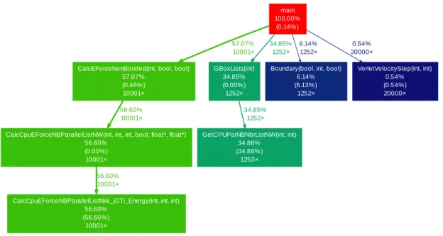
Figure3presents the profile of the sequential MOIL execution when simulating the Argon case study. It is possible to observe that the most time consuming routine is the CalcCpuEForceNB-ParallelListNW jGTi Energy. This routine is responsible by the calculation of the van der Waals forces that are exerted on a particle by the other particles, and takes 56.60% of the global execution time. The second most time-consuming routine is the GetCPUParNBNbrLis-tNWwhich builds the neighbors lists. In this case, the size of the problem is small, which means that the calculation of the forces finishes faster, which implies a smaller ratio between the time spent in calculations and the time necessary to build the neighbors lists. In bigger problems this ratio would be larger, resulting in a larger percentage of time used to calculate forces. The other routines in the execution are much less time-consuming and only spend about10% of the global execution time. Thus, CalcCpuEForceNBParallelListNW jGTi Energy routine is the only one that needs to be improved for the biggest gain in performance.
main 100.00%
(0.14%)
CalcEForceNonBonded(int, bool, bool) 57.07% (0.46%) 10001× 57.07% 10001× GBoxLists(int) 34.85% (0.00%) 1252× 34.85% 1252×
Boundary(bool, int, bool) 6.14% (6.13%) 1252× 6.14% 1252× VerletVelocityStep(int, int) 0.54% (0.54%) 20000× 0.54% 20000×
CalcCpuEForceNBParallelListNW(int, int, int, bool, float*, float*) 56.60% (0.00%) 10001× 56.60% 10001× GetCPUParNBNbrListNW(int, int) 34.88% (34.88%) 1253× 34.85% 1252×
CalcCpuEForceNBParallelListNW_jGTi_Energy(int, int, int) 56.60%
(56.60%) 10001×
56.60% 10001×
Figure 3.: Profiling of the Argon simulation in MOIL with the dynaopt tool.
Before the execution of the main steps of the MD simulation, MOIL performs several initial-ization steps. The initialinitial-ization steps include reading two files, one with the coordinates of all particles in the system and the other with the characteristics of the particles and the simulation parameters, such as the total number of simulation steps and the number of steps between the neighbors list update of each particle.
3.2. MD Sequential Version
After identifying the initialization steps performed in MOIL, the most important data structures were analyzed. The structures are used to store forces, velocities and positions. These three vector quantities are saved in nine arrays, since each one has three components: (Qx, Qy, Qz). These arrays are filled after certain validations and are obtained from data structures implemented in Fortran that are shared by several MOIL tools. In the Argon case study, the neighbors list of all particles is updated every three steps. All the MOIL data structures, such as the neighbors lists, are built from the mentioned nine arrays.
The code of the routine that calculates the forces exerted on each particle uses a neighbors list, as it can be seen in listing3.1 (full for in listingA.1). The list of neighbors of a given particle includes all the particles that are within a certain radius around that particle. The routine iterates over this list to obtain the index of a neighbor particle. This index is then used to get the neighbor particle coordinates from the array of coordinates. With the coordinates of two particles, it is then computed the force exerted between them. This means that there are two steps to get a particle coordinates: first it is obtained the index of the particle and later are read the coordinates of the neighbor particle. Next, the routine checks if the particle is inside the given radius. If true, the force between the particles is calculated and its value is stored in the forces array, on the position corresponding to the particle being processed.
The calculation of a force is always done between two particles: (i) the principal particle, the one that accumulates the forces exerted by all its neighbors, and (ii) the neighbor particle, the one that calculates only the force exerted by the principal particle. Because this implementation uses the third law of Newton, while the principal particle is accumulating the force exerted on it by all its neighbors, the force exerted by the principal particle on the neighbor is also updated. This reduces the number of forces calculated by the routine, but it introduces an additional complexity due to the necessity to exclude the principal particle from the neighbors list of its neighbors.
// Iterate over all particles
for (int a=0; a<pend; a++) {
//Number of neighbors for particle a nnbrs = nrNbrAtomsPar[a];
...
// Iterate over the particle neighbors
for (int n=0; n<nnbrs; n++) {
// Get neighbor information from the structure
3.2. MD Sequential Version
// Index of the neighbor in the array of coordinates j = nbr.x;
...
if (r2 < UCell.dMaxInnerCut2) {
// Calculate vdW force using LJ
r =sqrt(r2); invr2=1.0f/r2; invr6=(invr2*invr2*invr2)*valid; FLJ=-12.0f*nbr.y*invr6*invr6*invr2+6.0f*nbr.z*invr6*invr2; // Calculate energy
Evdw = (nbr.y * invr6*invr6 - nbr.z * invr6);
float df = FLJ - Fe;
// Accumulate forces exerted on a particle AtiFx += df*rx; AtiFy += df*ry; AtiFz += df*rz; // Subtract particle force of the neighbor particle StoreXDP[j + cpuForceSpacing*tid] -= df*rx;
StoreYDP[j + cpuForceSpacing*tid] -= df*ry; StoreZDP[j + cpuForceSpacing*tid] -= df*rz; ELJ += Evdw; EElec += Eel; } ... }
Listing 3.1: For cycles that calculate the forces exerted on each particle by its neighbors.
After the code analysis it was decided to extract the core code of the MD simulation to a simpler and separated implementation. This decision was taken because, as it was mentioned before, MOIL was first developed using Fortran language and only afterwards ”converted” to C. This resulted in a mixed implementation using Fortran and C, where the main routine does a lot of validations and becomes disorganized. Such an example of code disorganization is the branch that tests what is the current iteration before relocating the particles and rebuilding the neighbors lists. Therefore, to facilitate the implementation of code optimizations it was used the JGF MD benchmark (Smith et al.,2001). This benchmark is used in the university and provides an easier infrastructure for development. The JGF MD benchmark does not use neighbors lists or any domain division. This code uses third law of Newton to reduce the computations of forces. The purpose of the JGF version is to execute the MD simulation without using neighbors lists and to
3.3. MD Vectorization
allow us making modifications more easily. The changes made to JGF were in the computation of forces and the type of arrays to use a structure similar to the MOIL package. The values of the coordinates in JGF were saved as doubles while MOIL uses floats. After these changes the development with the JGF MD benchmark was similar to the one performed with MOIL. First we analyzed the code, identifying the most time-consuming routine, and then the code was changed to improve its performance.
3.3 M D V E C T O R I Z AT I O N
Vectorization is a process of converting a scalar instruction, which process a single pair of operands at a time, to one where a single operation is applied to multiple elements (SIMD paradigm). This form of parallelism is called data parallelism. The processors that support these type of operations are called vector processors. One of the first processors supporting these op-erations was the Cray 1 (Russell,1978). Recently, there was a growth of new technologies, such as AVX and AVX2, that support vectorization. The vectorization extension used in this thesis is AVX, which was introduced with the Intel Sandy Bridge micro-architecture. The AVX instruc-tion set extension increased the width of the registers from 128- to 256-bit. This means that AVX made it possible to execute 4 double precision FLOP per cycle or 8 single precision FLOP per cycle. These operations increase the number of operations per cycle, reduce the number of cycles, and reducing the best case execution time by 8 times.
The process of transforming sequential to vectorized code is a hard task to be done manually. That is why it is so important that compilers automatically do this transformation. This depends on the calculations and the used data structures, but most of the essential changes are related with conditional expressions and arrays. The conditional expressions, like if conditions, have to be removed to allow the compiler to apply vectorization. Arrays are important and essential. Using arrays will allow multiple array elements to be processed in a single cycle. The changes related to arrays accesses are dictated by (i) the way arrays are aligned in memory, (ii) the knowledge the compiler has over the pointers to arrays, and (iii) how arrays are accessed by the application. If an array is not aligned, or the pointer to that array has the possibility of being an alias for other array, then the compiler cannot use vectorization. In this case there is a need to manually specify that the alias is restricted to that array and it is not used in another array. The way we access arrays also has to be known by the compiler. All accesses have to be aligned, the array positions have to be known at compile time, and have a stride 1 access with being depending on
3.3. MD Vectorization
conditions. For example, considering a for cycle that increases its counter by one, if we access an array based on this counter then the compiler will know the accessed array positions and it will be able to vectorize the calculations involving the array.
3.3.1 Code modifications
The code used in the present dissertation had the problems explained above. The if conditions present in the code were used to verify if the coordinates of a particle are still inside of the sim-ulation box and if that particle is within a distance (or radius) valid to calculate forces. The first conditions alter the coordinates of the particle in a way that if its outside the simulation box it is replaced inside the box, by applying the periodic boundary conditions (PBC). This can be seen in the listing3.2that shows three if conditions that compare the distance between both particles
co-ordinates (rx,ry,rz) with the limits of the simulation box (±cellxhlf, ±cellyhlf,
±cellzhlf). The condition present in listing 3.3 is used to test if the neighbor particle is inside the cut-off radius of the particle being calculated. This condition has to exist because the update of the neighbors lists positions is only done after a few iterations, which means that while the lists are not updated, the neighbor particle can move to outside the radius. Both conditions explained before produce many conditional jumps, which can be seen in the associated assembly code. This prevents the compiler to do automatic vectorization.
if (rx > cellxhlf) rx -= cellxhlf*2.0f else if (rx < -1.0f*cellxhlf) rx += cellxhlf*2.0f; if (ry > cellyhlf) ry -= cellyhlf*2.0f;
else if (ry < -1.0f*cellyhlf)
ry += cellyhlf*2.0f;
if (rz > cellzhlf) rz -= cellzhlf*2.0f;
else if (rz < -1.0f*cellzhlf)
rz += cellzhlf*2.0f;
3.3. MD Vectorization
r2 = rx*rx + ry*ry + rz*rz;
if (r2 < UCell.dMaxInnerCut2) {
... // Force and energy calculation }
Listing 3.3: Conditional statement related with the cut-off distance.
The solution to perform vectorization was to remove both sets of conditional statements from the code. To remove these conditions we took advantage of two aspects: (i) the evaluation of a boolean expression in C is 0 or 1, and (ii) the calculations controlled by the conditions are accumulative, which allow us to multiply the result of the boolean condition evaluation by the value that must be accumulated in the variables. The condition removal, using this technique, can be seen in the listing3.4. It is possible to see in this listing that the conditions are converted in calculations that were further split in two smaller calculations. The division of the calculations had to be done because if these calculations were done in a single instruction, the compiler would produce the same assembly code as in the original conditions. In such case the compiler would interpret the calculation as a conditional statement and it will not vectorize the code. The same approach was used to remove the condition present in listing 3.3. In this case the unique differ-ence is the condition evaluation result (0 or 1) being stored directly in the variable valid that is used in all calculations inside the removed if statement. If the result is 0 the particle is outside the cut-off radius and if is 1 the particle is inside of it. The first set of conditions (listing 3.2) does not introduce new calculations, because the adjustment made inside each condition only alters a single variable in a single calculation. In contrast, the replacement of the conditional statement present in listing 3.3 introduces more calculations because in this original code the condition body instructions are only executed when the condition is true, and in the replacement code (listing3.5) the the condition body instructions are always executed. This means that when the result of the condition evaluation is false the condition body instructions cannot alter the re-sult of the simulation. Since in listing 3.5 the calculations made inside the condition body are always accumulated, when the condition is evaluated to false the calculations of the force and energy must be both zero. This is true because the expressions that compute the force and energy are both multiplied by valid=0, which ensures the necessary null result that will not change the accumulated values of the force and energy.
3.3. MD Vectorization cellxhlfm=-1.0f * cellxhlf; cellyhlfm=-1.0f * cellyhlf; cellzhlfm=-1.0f * cellzhlf; ... rx += (rx > cellxhlf) * (cellxhlfm*2.0f); rx += (rx < cellxhlfm) * (cellxhlf*2.0f); ry += (ry > cellyhlf) * (cellyhlfm*2.0f); ry += (ry < cellyhlfm) * (cellyhlf*2.0f); rz += (rz > cellzhlf) * (cellzhlfm*2.0f); rz += (rz < cellzhlfm) * (cellzhlf*2.0f); r2 = rx*rx + ry*ry + rz*rz;
valid = (r2 < UCell.dMaxInnerCut2)
Listing 3.4: Removing conditional statements present in listing3.2to allow vectorization.
valid = (r2 < UCell.dMaxInnerCut2) // Calculate vdW force using LJ
r = sqrt(r2); invr2 = 1.0f/r2; invr6 = (invr2*invr2*invr2) * valid; FLJ = -12.0f * nbr.y * invr6*invr6*invr2 + 6.0f * nbr.z * invr6*invr2; // Calculate the energy
Evdw = (nbr.y * invr6*invr6 - nbr.z * invr6);
Listing 3.5: Removing conditional statement present in listing3.3to allow vectorization.
After having a modified code that is prepared for vectorization, it was analyzed using the PAPI. Figure4presents the number of executed instructions, with and without the if conditions. It is possible to observe that when a set of if conditions is removed the total number of instruction increases, while the number of branch instruction reduces. This happens because with the re-moval of both sets of if conditions, the calculations are always done, even if the if conditions are evaluated to false.
3.3. MD Vectorization
#Instruc)on #Clock Cycles #Intruc)ons Load #Instruc)ons Store #Intruc)ons Branch
Original 7324301 6042425 2150288 393927 541405 Without if Valid 8954085 6893777 2588598 522508 495608 Without if rx,ry,rz 8278997 7144699 2657639 391846 176314 0 1000000 2000000 3000000 4000000 5000000 6000000 7000000 8000000 9000000 10000000
Figure 4.: Number of instructions run in the original MOIL code and in the code modified for vectoriza-tion.
The original routine used to compute the forces had several problems related to the used data structures. To access arrays it was used an alias that the compiler did not know if it belongs to another array. This prevents vectorization. The problem was solved by applying the keyword restrict. Another problem came from the way arrays were accessed to update the forces. The positions within the arrays were accessed in an irregular way inside a cycle. The irregular array accesses occurred when MOIL uses neighbors lists and the index of the next neighbor point to a random position in the array of coordinates. In this case, the simpler way to enable automatic vectorization is to access the arrays according to a cycle counter.
Both the modifications to MOIL and JGF MD benchmark, to enable vectorization, resulted in no gains. The main reason was the small number of instructions that could be vectorized by the compiler in comparison with the added instructions overhead resulting from the removal of the conditional statements. To overcome this overhead it was decided to develop an organization of particles in cells which will be explained bellow.
Implementation of cells
The cells are implemented using an array of structures, where the structure is a cell and has the information of all particles in that cell and each index of the array is a cell. It is also necessary to
3.3. MD Vectorization
create an array for each cell that has the index of its neighbors. Using an array of structures and neighbors we need to iterate through 4 different arrays to compute the forces. These arrays are, (i) array of cells, (ii) array of particles in the cell, (iii) array of the neighbors cells and (iv) the array of the particles of the neighbor cell. To iterate over all these arrays it is needed four loops, one for each array. With the introduction of these loops the compiler can apply vectorization to a larger number of instruction, if the accesses to these arrays are stride 1.
The first step was to create a data structure to store the particles of the cells and to distribute the particles by the created cells. After creating the cells, it was necessary to create a list of neighbors cells. This list is necessary to compute forces among particle that are close to the limits of a cell. Concretely, accessing neighbor cells is necessary when there are particles in different cells separated by a distance smaller than the cut-off radius. In this case, to compute the force exerted on such a particle we have to access some particles located in neighbor cells. To construct the list of neighbor cells we have to identify all cells that are adjacent to each cell in three-dimensional space. Since the cells are cubes, one cell has a maximum of 26 neighbor cells. Building the list of neighbor cells has to be done carefully because of two reasons. First, to find the neighbors of a cell located in the limits of the simulation box we have to apply PBC. Consider that a cell is identified by a 3D coordinate (cidZ,cidY,cidX). If the coordinate has a component with the maximum or minimum allowed value, for examplecidXis equal tocidmax orcidmin, the PBC means that there is a neighbor cell with a X coordinate equal to the minimum (cidmin) or maximum (cidmax) allowed value. Second, as we use Newton’s third law, it implies that if a cell B is in the neighbor list of cell A, then A can not be on the neighbor list of B. This means that the particles of cell A need not be used explicitly to calculate the forces exerted on the particles of B, because these forces have already been calculated when the particles of A were processed. When the cell data structure was designed, the function responsible for calculating the forces had to be modified to use this new structure. In the listing 3.6 we can see the introduction of new cycles to iterate over the different cells and particles. The new cycles made it possible to have a greater number of vectorized instructions.
for ( Iterate over all cells ) // (C) {
for ( Iterate over all particles of the cell ) // (CP) {
// Read cell particles and forces arrays ...
for ( Iterate over all neighbor cells ) // (CN) {
3.3. MD Vectorization
// Read neighbor cell particles and forces arrays ...
for ( Iterate over the neighbor cell particles) // (CNP) {
// Calculate forces exerted on the particle ...
// Store component X,Y,Z of force ForceX[CNP] -= (Calculated Force X); ...
// Accumulate component X,Y,Z of force AccumulateForceX+= Calculated Force ...
} }
// Store component X,Y,Z of force ForceX[CP] += AccumulateForceX; ...
} }
Listing 3.6: For cycles that calculate the forces using cells.
After having the first MD implementation with cells, the next phase was to vectorize the code that uses the cell data structures. When using cells we have 4 different cycles that access arrays and make calculations with data from these arrays. Vectorizing the inner cycles will allow the conversion (vectorization) of a large number of instructions. The principal problem of the cells version is when the accesses to the array of forces, in the inner loop, is not stride 1. This happened in the application of the third law of Newton. The problem was solved by storing the forces in an array local to each cell, in the position corresponding to the neighbor particles. When all calculations are finished, the local forces are added to the respective position in the three global arrays of forces. With these modifications a large number of instructions was vectorized automatically by the compiler, in the same way as explained in previous section.
With all optimizations implemented in the version using cells, this version was compared with the original one using PAPI. Figure 5 shows that the number of instructions executed in the non-vectorized version using cells is much larger than in the code without cells. The code with vectorization has a number of instructions close to the original version, since the increase in in-structions is compensated by the use of vector inin-structions. The number of executed inin-structions
3.3. MD Vectorization
increases strongly when we use cells due to (i) removing the cut-off conditional statement in-troducing additional calculations made for particles that are inside a cell but outside the cut-off radius and (ii) the additional allocations that we had to do. It is also possible to observe that the number of clock cycles using vectorization is smaller than in the original code, which means that the vectorized cell version is faster than the original.
#Instruc)ons #Clock Cycles #Load Intruc)ons #Store Instruc)ons Intruc)ons #Branch Original 6942192 5887021 2194490 392563 543503 Cells (Vectorized) 7400699 5212980 2233031 475954 147213 Cells (Not Vectorized) 11932015 8469841 2895153 416929 138026 0 2000000 4000000 6000000 8000000 10000000 12000000 14000000
Figure 5.: Number of executed instructions and clock cycles in original MOIL code and in code with cells.
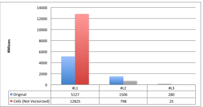
Using cells increases the number of instructions but the difference is reduced by using vectoriza-tion. Figure6presents the cache misses for both the original and cells versions. It is possible to see that with the introduction of cells the number of misses increases. This happens because the original code calculations only need a neighbors list of particles for each particle, while the code using cells needs a list of cells, a list of the particles inside the cell and a list of neighbor cells. This increases the size of the data that has to be loaded into the cache, resulting in misses in the first level of cache. However, the misses in the second level of cache reduces and it is even less that the original code. This reduction in cache misses is due to the cells being loaded as a block to the cache.
3.3. MD Vectorization #L1 #L2 #L3 Original 5127 1506 280 Cells (Not Vectorized) 12825 798 25 0 2000 4000 6000 8000 10000 12000 14000 #Mi ss es
Figure 6.: Cache misses comparison between the original version and the version using cells.
Figure 7presents the execution time for a single iteration over the whole simulation box. It is possible to see that using cells without vectorization slows down the execution, but with vector-ization we actually improve performance. This performance gain results from the fact that using vectorization we reduce the computation time needed for the calculation of forces.
3.4. Parallelization 0 0.0005 0.001 0.0015 0.002 0.0025 0.003 0.0035 0.004
Original Cells (Vectorized) Cells (Not Vectorized)
Ti
me (
s)
Figure 7.: Execution time comparison between original, not vectorized cells, and vectorized cells versions.
3.4 PA R A L L E L I Z AT I O N
3.4.1 MD Shared Memory Implementation
The first parallel version developed in this thesis used the shared memory model, via OpenMP. The objective was to parallelize the calculations done in the different cells but respecting the critical sections present in the code. To achieve this objective, it was necessary to introduce a change in the code presented in listing3.6. Inside the routine that computes forces there are two sections that need to be locked in order to avoid multiple thread accesses at the same time. One section is where the forces, calculated by the Newton laws, are written in the arrays. The other section is where the accumulated force of the principal particle is written in the arrays. These two sections are critical and should therefore be executed by a single thread at a time. The sections have to be locked because, even if every thread calculates only one cell, the calculation in that cell will need to read the particles of its neighbor cells and write the forces calculated into its neighbors cells particles, due to the third law of Newton. This means that every change to the cells arrays of forces, occurring inside the parallel region, must be locked to ensure that only one
3.4. Parallelization
thread can write in the arrays of forces at a time. Since we only want to lock the critical regions there are two ways to do it. The first way is to implement a lock by cell. Thus, a thread can write into a cell only if that cell is free. The second method implements a lock by particle. Here we lock the particle forces while a thread is writing. Both locking methods were implemented, using an array of locks, and tested. But the implementation using locks by particle prevented the compiler to perform vectorization. The lock by particle had to be implemented inside the cycle that calculates the forces, which means that it had to write in the array of locks in a calculated position that was not aligned. For this reason it was used locks by cell instead of particle.
3.4.2 MD Distributed Memory Implementation
Message Passing Interface (MPI) allows the developers to write portable message-passing code. MPI allows the data from one process to be moved to other processes in a high level and abstract way. The communication between processes is known as a distributed memory communication environment.
When using OpenMP, for example, there is a limitation in the available resources because it only allows to create threads inside a single machine, but MPI expands the available resources because it allows the processes to communicate between different nodes in a easy and abstract way. This means that if there are no bottlenecks, the performance of a program can be improved by using more nodes.
Comparing with the previously presented MD versions, the development of the MPI version placed less challenges. This is due to the fact that all forces are accumulative, which creates no problems to the task of writing the forces in the arrays. The approach followed in the MPI implementation consisted in having several cells allocated to each process. This way, one process calculates the forces in different cells and adds them to its local array of forces, in the same way as referred before. After this, all processes communicate their forces to the other processes that add them to their own arrays. Using MPI this operation can be done using a reduction of the forces followed by a broadcast of the result (all-reduce). This approach avoids several problems of the shared memory model such as the necessity to block the critical sections.
3.4. Parallelization
3.4.3 MD Hybrid Implementation
The MD hybrid version consisted in using both the shared and distributed memory models in the implementation. This implementation eliminates the main limitation of the OpenMP code since the available resources are not limited to a single node. The MPI implementation had already solved this limitation, but an hybrid implementation allows a much higher performance in some cases. For example, when there is a lot of communication between processes and when there are few critical sections. In our code we benefit a little from each model. We can reduce the time spent in communication, because we have less processes that need to communicate, we also use less memory space because with threads it uses shared memory and because we have few critical sections the execution seldom blocks in these sections.
The hybrid implementation simply combines the OpenMP with the MPI implementation, while ensuring that the critical sections and the cell organization are respected.
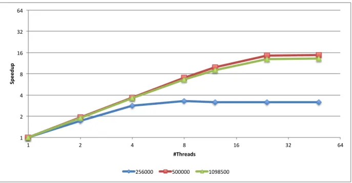
There are many ways to assess an hybrid implementation in order to reach the best performance. It is possible to test the code with different combinations of the number of threads, the number of processes, and how to distribute processes and threads by nodes. Different combinations were tested in this work. The alternatives that resulted in best performance will be documented in the next chapter.
4
R E S U LT SIn this chapter it is presented the results obtained with the different implementations. The results in this section are obtained using the Argon case study with different numbers of particles.
4.1 T E S T E N V I R O N M E N T
In order to evaluate the development made in this thesis the Services and Advanced Research
Computing with HTC/HPC (SeARCH) cluster was used (University of Minho, 2015). It was
also used various tools (table 1). The specifications of the nodes used in the simulations are in table2.
Table 1.: Tools used for development.
Tool Version Description
GNU gprof 2.25 Used to obtain the profiles of the code with the
correspond-ing weights of of each routine.
GCC 4.9.0 The compiler used in most of the implemented code.
OpenMPI 1.8.2 MPI version.
4.2. Case Study
Table 2.: Specifications of the nodes used in simulations.
Node compute-662 Processor
Model: Intel(R) Xeon(R) CPU E5-2695 v2 @ 2.40GHz
Thread(s) per core: 2
Core(s) per socket: 12
CPU socket(s): 2 NUMA node(s): 2 CPU MHz: 2400.000 L1 data cache: 32K L1 instruction cache: 32K L2 cache: 256K L3 cache: 30720K Other Ram Size 64GB OS Rocks 6.1 CentOS 6.3 4.2 C A S E S T U D Y
The case of study used in all presented results is a cube of Argon atoms. The measurements were made using cubes with different number of particles, while keeping the same cut-off in all versions. The number of used particles are presented in table3.
Table 3.: Number of particles used in the MD simulations.
Number of particles Memory space to save the coordinates of particles
864 20.25KB 2058 48.23KB 8788 205.96KB 19562 458.48KB 256000 5.86MB 500000 11.44MB 1000000 22.88MB
The utilization of different numbers of particles aimed to have data sizes that could fit in different levels of cache. The domain (simulation box) size of the input increases when the number of particles increases, given that the density of particles is maintained constant.
4.3. MD Sequential Versions
4.3 M D S E Q U E N T I A L V E R S I O N S
The simulation results documented in this section were obtained with a developed sequential code that is similar to MOIL.
In table 4 are presented the measurements of three versions of the sequential code. The first two differ on how the coordinates are saved, one uses floats to save the particles positions while the other version uses doubles. The reasons for this measurements are, that MOIL uses floatsto save its coordinates while in JGF they are saved as doubles and also because with coordinates as doubles there are limitations in vectorization. These two reasons brought the need to use floats instead of doubles to see their performance differences. The third version is also implemented with floats and cells.
Table 4.: Execution time in seconds of the MD sequential versions.
# Particles Sequential version (floats) Sequential version (doubles) Sequential with cells
864 0.0116 0.0072 0.0146 2048 0.064 0.0396 0.0821 8788 0.6932 0.5188 1.4745 19652 2.4564 1.9834 7.2932 256000 258.6384 236.6036 155.0428 500000 936.1647 870.1428 250.9159 1098500 4317.2459 4089.8578 621.1615
The floats version has a small overhead due to the conversion between floats and doubles. While the coordinates could be converted to float, the forces cannot be converted to float because they are calculated and need to have double precision. This means that the calculations of the distance between particles are done with floats, which are then used in the calculation of forces, being the results saved in double precision.
The performance improvement that results from using cells can only be seen when we increase the number of particles to 256000. This increase in performance only happens because with the input used, the particles are close to each other forming a dense system which means that only after reaching this number of particles it is possible to have more than 27 cells with the used cut-off distance. When the domain can only be subdivided in 27 cells or less, the calculation of forces is done in the same way as the other versions, without cells, but with a time overhead due to cell construction.
4.4. Vectorized MD
4.4 V E C T O R I Z E D M D
Vectorization solves most problems of the sequential versions. The conversion between floats and doubles can be completely ignored because the compiler, after calculating the floats in a single instruction, can store all results (as doubles) without extra instructions for data type conversion.
The implementation of celss with vectorization outperforms all other versions for all the input sizes. Without using cells the compiler can only vectorize a small number of instructions because of the way the forces are calculated. The results obtained with the vectorized version without cells, as they did not allow performance improvement, are not presented. With cells, the compiler can produce a larger number of vectorized instructions achieving a greater performance improve-ment. In figure8it is possible to see that for the largest domain size, the vectorized version with cells is about 29 times faster than the sequential version with doubles (original one) and it is about 4 times faster than the non-vectorization version using cells.
0 500 1000 1500 2000 2500 3000 3500 4000 4500 5000 256000 500000 1098500 Ti me( s) #Par-cles
Sequen0al Version (floats) Sequen0al Version (doubles) Sequen0al with Cells Vectorized with Cells
Figure 8.: Sequential versions execution time.
We have seen that the code with cells, but without vectorization, was slower than the original version for smaller domain sizes. When we vectorize the code with cells, we get better perfor-mance than the original one, for all input sizes. We can then conclude that vectorization is quite advantageous if we use cells.