Setembro, 2016
CHARACTERIZATION OF THE TURBULENT
STRUCTURE IN COMPOUND CHANNEL FLOWS
Dissertação para obtenção do Grau de Doutor em Engenharia Civil
Orientador: João Gouveia Bento Aparicio Leal,
Assistant Professor, FCT/UNL, Portugal
Professor, Universitetet i Adger, Norway
Co-orientador: Luis R. Rojas
–
Solórzano
Associate Professor
Nazarbayev University, Kazakhstan
Nº de
[Characterization of the Turbulent Structure in Compound Channel Flows]
Copyright © Ricardo Manuel Martins de Azevedo, Faculdade de Ciências e Tecnologia,
Universidade Nova de Lisboa.
i
Acknowledgments
I would like to thank the Faculty of Science and Technology of New University of Lisbon
(FCT/UNL), for accepting me as PhD student. I would like also to acknowledge the University
of Beira Interior for providing the necessary conditions to carry out this work.
To my supervisors, Prof. João Leal and Prof. Luis Rojas, for accepting me as a PhD
student, for all the dedication and guidance fundamental for the development of this thesis, for
all the patience, support, encouraging, and especially for all the knowledge provided. It is a
pleasure to work with you! Thank you!
A special gratitude to Prof. Rui Ferreira for his assertive and invaluable advices and help
about data processing and turbulence process understanding. Prof. Koji Shiono deserve a special
mention for advising me in turbulent flows and LDV measurements. To Prof. Cristina Fael for
receiving and providing the necessary conditions at University of Beira Interior.
To Jorge Barros for all the help, support, patience and encouragement when LDV was
damaged and I began to get in stress. But above all, thank you for your friendship during this
process. You are part of my family! I will be always in gratitude with you.
My thanks to Marina Filonovich for your help, support and understanding. João
Fernandes for bring me your help in the filtering data process and Moisés Brito for work with
me in the analysis of algorithms built to estimate the turbulent scales and dissipation rate.
Special thanks to Jorge "El Melenu'o" de Oliveira, Alita "La Abuelita" Amorim and Sara
"La Doctora" Amorim for your support, advices and relaxing time during this process and
especially for all the barbecue and parties moments.
I would also like to express my deep gratitude to my fiancée Manuela Amorim for all the
support, encouragement, and help, especially in this last months, to finish this work. Probably,
without your presence, this thesis never would be written and this chapter of my life never
would be enclosed.
To my parents and sister for all the support through my entire carrier as a student and as
investigator. All that I have and I am today, I owe to you. Many thanks!
This work was supported by National Funds from the Foundation of Science and
Technology (FCT) through the scholarship SFRH/BD/33646/2009 and through the projects
iii
Abstract
The main goal of this investigation is to characterize the turbulent structures in compound
channel flows considering two geometrical conditions, a simple asymmetric compound channel
and the same compound channel but with the placement of rods on the upper bank.
For the simple asymmetric compound channel, three different water depths were
analyzed, one corresponding to deep flows and two corresponding to shallow flows. For the
compound channel with rods, three different spacing between elements were studied, including
two different water depths for each spacing condition.
The measurements were taken with a 2D Laser Doppler Velocimiter, at 9.0 m from the
inlet for simple compound channel. For the compound channel with rods, three cross-section
around 9.0 m from the inlet of the channel were measured, corresponding to locations
downstream of the rod, in the middle of two rods and upstream of the rod. The measurements
were performed under quasi-uniform flow condition and streamwise and vertical instantaneous
velocity components were obtained.
The raw data was filtered and processed in order to estimate the time-averaged
velocities U and W, the turbulent intensities U' and W', Reynolds stress u'w', streamwise integral length scale Lx, turbulence dissipation rate ε and Taylor’s micro scale x. Taylor's frozen field hypothesis was adopted in order to transform the time record into a space record, using a
convection velocity Uc. The autocorrelation function was built and the integral length scale estimated using three different stop methods of the integral: the second zero of the
autocorrelation function, the first minimum, and assuming the integral length scale as
the wavenumber value when the autocorrelation function reaches 1/e (this was concluded to be
the most consistent method). For estimating the dissipation rate, the following methods were
used: from the third order structure function, from the second order structure function and
finally, and from the energy spectrum of the velocity (this was concluded to be the most
consistent method).
In the case of a simple compound channel, the deep flows are characterized by macro
vortices with streamwise axis between the interface and main channel and between interface and
floodplain, having a notable separation in the "main channel vortex" and the "floodplain
vortex" meeting, due the double shear layer of the streamwise depth-averaged velocity. Shallow
flows are characterized by macro vortices with vertical axis confined between the interface and
main channel and originated by the depth average velocity gradient between the main channel
iv
fully developed open-channel flow equations that relation appears to be constant for all
water depths.
For the compound channel with rods, new turbulent structures are generated due the
interaction between rods and flow. Downstream of rods, the horseshoes-vortex system is
perfectly observed and a strong descendant flow dominate both sides of rod, turning invalid the
universal laws for 2D fully developed open-channel flows. The integral length scale presents
almost constant values in the vertical direction, which indicates that the wakes generated by the
rods influence the entire water column. The turbulent microscale and dissipation rate acquire a
streamwise variation due to the vortex propagation in the downstream direction, both presenting
higher values than the ones corresponding to 2D flows.
v
Resumo
O principal objetivo desta investigação é a caracterização das estruturas turbulentas em
escoamentos em canais de secção composta tendo em consideração duas condições geométricas:
um simples e outro com elementos cilíndricos na parte superior do talude.
Para tal, três alturas diferentes de água foram analisadas para o caso do canal simples, uma altura correspondente a escomento profundos “deep flows” e dois relativos a escoamentos rasos “shallow flows”. Para o canal composto assimétrico com elementos cilíndricos, foram
estudados três espaçamentos entre cilindros e duas alturas de água para cada um dos
espaçamentos. Os espaçamentos estudados foram S1 = 1m; S2 = 0.2m; e S3 = 0.04m, e os elementos cilíndricos colocados foram barras de alumínio de 0.01m de diâmetro e 0.1m de
comprimento.
Foi utilizado um Laser Doppler Velocimeter 2D para a realização das medições, as quais
foram realizadas a 9.0m da entrada do canal composto simples. No caso do canal composto com
elementos cilíndricos, foram medidas três secções transversais localizadas nas proximidades de
9.0 m desde a entrada, sendo uma secção medida à jusante do elemento, outra secção no meio
de dois elementos e a última a montante do elemento cilíndrico. As medições foram executadas
em condições de escoamento quasi-uniforme, obtendo-se as velocidades instantâneas das
componentes longitudinal e vertical.
Depois de medir a secção transversal, os dados foram filtrados e processados de forma a
obter uma estimativa da velocidade média temporal U e W, das intensidades turbulentas U' e W',
tensões de Reynolds u'w', da macro escala longitudinal Lx, da taxa dissipativa longitudinal εx e
da micro escala de Taylor's longitudinal x. Para isso, adotou-se a hipótese de Taylor de forma a
transformar o registo temporal num registo espacial com a implementação de uma velocidade de
convecção Uc. Neste sentido, a função de autocorrelação foi construída, podendo-se estimar o
comprimento da macro escala "integral length scale" utilizando três métodos para definir o
limite superior da integral, nomeadamente, encontrando o segundo zero da função de
autocorrelação; encontrando o primeiro mínimo da função de autocorrelação; e assumindo o
valor da macro escala integral como o valor do número de onda quando a função de
autocorrelação atinge 1/e. No caso da taxa de dissipação, foram utilizados três métodos. A
estimativa da taxa de dissipação através da função de estrutura de terceiro ordem, através da
função de estrutura de segundo ordem e, finalmente, a partir do espectro da velocidade. A micro
escala longitudinal de Taylor foi estimada como uma função da taxa de dissipação turbulenta,
assumindo um escoamento turbulento isotrópica homogénea incompressível.
No caso do canal composto simples, os escoamentos profundos "deep flows" são
caracterizados pela existência de macro vórtices de eixo longitudinal entre a zona da
vi
notável na confluência entre o vórtice do leito principal "main channel vortex" e o vórtice da
planície de inundação "floodplain vortex", devido à dupla camada limite da velocidade média
em profundidade. Os escoamentos rasos "shallow flows" são caracterizados por macro vórtices
de eixo vertical confinados entre a interface e o leito principal, os quais são originados pelo
gradiente da velocidade média em profundidade entre o leito principal e a planície de
inundação.
Para o canal composto com elementos cilíndricos, novas estruturas turbulentas são
geradas devido a interação entre estes elementos e o escoamento. A jusante das hastes, o sistema
de vórtices em forma de ferradura "horseshoes-vortex system" é perfeitamente observada e um
forte fluxo descendente domina o escoamento em ambos os lados da haste. No entanto, este
processo é dissipado na direção longitudinal, onde o comportamento do escoamento começa a
exibir uma maior interação entre a planície de inundação e o leito principal, até chegar ao
vii
Table of Contents
CHAPTER 1 ... 1
INTRODUCTION ... 1
CHAPTER 2 ... 7
LITERATURE REVIEW ... 7
2.1. DIFFERENTIAL CONSERVATION EQUATIONS ... 10
2.1.1 Momentum balance equation for compound channel flow ... 13
2.2 MODELING OF TURBULENCE ... 14
2.2.1 Statistically Stationary Processes ... 15
2.2.2 The energy cascade and Kolmogorov hypotheses ... 19
2.2.3 Taylor's or Frozen-Field Hypothesis ... 24
2.2.4 Structure Functions ... 25
2.2.5 Taylor microscales ... 28
2.2.6 Dissipation Rate ... 29
2.3 TWO-DIMENSIONAL FLOW STRUCTURES ... 30
2.3.1 Flow Velocity ... 30
2.3.2 Turbulence Intensity ... 33
2.3.3 Effect of rough beds ... 34
2.3.4 Integral length scale of eddies ... 37
2.3.5 Microscale of eddies ... 38
2.3.6 Dissipation rate of turbulent energy ... 39
2.3.7 Shear or Friction Velocity ... 40
CHAPTER 3 ... 43
EXPERIMENTAL SETUP AND MEASURING ... 43
3.1 EXPERIMENTAL SETUP ... 45
3.1.1 Roughness Coefficient ... 46
3.2 MEASURING TECHNIQUE: LASER DOPPLER VELOCIMETER ... 48
3.2.1 Probe Calibration... 51
3.2.2 FlowSizerTM Software ... 53
3.3 SEEDING PARTICLES CHARACTERISTICS USED FOR LDV SYSTEM ... 56
3.4 EXPERIMENTAL CAMPAIGN ... 59
3.5 DATA ACQUISITION AND PRE-PROCESSING ... 65
3.5.1 Spike Replacement ... 66
CHAPTER 4 ... 69
viii
4.1 INFLUENCE OF THE SIDEWALL EFFECT ON ASYMMETRIC COMPOUND CHANNEL FLOWS 71
4.1.1 Introduction ... 72
4.1.2 Experimental Setup ... 73
4.1.3 Results and Analysis of Results ... 76
4.1.4 Conclusions ... 80
4.2 EXPERIMENTAL CHARACTERIZATION OF STRAIGHT COMPOUND-CHANNEL TURBULENT FIELD ...81
4.2.1 Introduction ... 81
4.2.2 Experimental Setup ... 82
4.2.3 Results and Discussion ... 83
4.2.4 Conclusions ... 91
4.3 INFLUENCE OF VEGETATION ON COMPOUND-CHANNEL TURBULENT FIELD...92
4.3.1 Introduction ... 92
4.3.2 Experimental Setup ... 93
4.3.3 Results and Discussion ... 94
4.3.4 Conclusions ... 105
4.4 TURBULENT STRUCTURES, INTEGRAL LENGTH SCALE AND DISSIPATION RATE IN COMPOUND CHANNEL FLOW ... 107
4.4.1 Introduction ... 107
4.4.2 Experimental Setup ... 109
4.4.3 Methodology ... 112
4.4.4 Results ... 117
4.4.5 Conclusions ... 124
CHAPTER 5 ... 127
CONCLUSIONS AND FUTURE RESEARCH ... 127
APPENDIX A ... 137
CODES TO DATA PROCESSING ... 137
ix
List of Figures
Figure 1.1 Number of floods by decade (Millennium Ecosystem Assesment) ... 3
Figure 2.1 Flow field associated with a straight compound channel (Shiono and Knight, 1991). ... 14
Figure 2.2 Ensemble of repeated experiments under similar initial a boundary conditions. (Tropea et al., 2007) ... 15
Figure 2.3 Mean
U
t
(solid line) and variance var(u)u'
t 2 from three repetitions of a turbulent-flow experiment (Pope, 2000) ... 16Figure 2.4 a) Sine function. b) Narrowband random noise. c) Broadband random noise ... 17
Figure 2.5 The integral-stop-values used to determine the macro-scale.
rx autocorrelation function; rx intervals of space in the longitudinal direction (Tropea et al., 2007). ... 18Figure 2.6 Schematic representation of the Energy Cascade. ... 22
Figure 2.7 Turbulence generated through a grid. b) Development of the different stages of the turbulence. Stage(i) Transition to a fully developed turbulent flow. Stage (ii) and (iii) Fully developed turbulent flow. Stage (iii) Dissipation of the smallest eddies. ... 23
Figure 2.8 Variation of the kinetic energy for the different stages of flow. ... 24
Figure 2.9 Sketch showing the points x and x+r in terms of x(n) and y(n). ... 25
Figure 2.10 Second-order velocity structure functions. Horizontal lines show the predictions of the Kolmogorov hypotheses in the inertial subrange, eqs. 2.51 and 2.52. (Pope, 2000) .... 27
Figure 2.11 Evaluation of Taylor's microscale. Tropea et al. (2007) ... 29
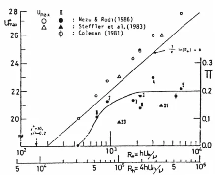
Figure 2.12 Wake strength parameter and maximum velocity Umax as functions of Reynolds number Re* and Reh. Nezu and Nakagawa (1993) ... 32
Figure 2.13 Sub-division of the flow field in open channels (cf. Nezu and Nakagawa 1993). ... 33
Figure 2.14 Turbulent flow over smooth and rough beds. a) Smooth bed. b) Rough bed. Nezu and Nakagawa (1993) ... 35
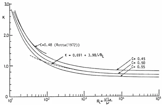
Figure 2.15 Variation of coefficient K against the Reynolds number RL. Nezu and Nakagawa (1993) ... 37
Figure 2.16 Distributions of Taylor’s micro-scale H varying Reynolds and Froude numbers. Nezu and Nakagawa (1993) ... 39
Figure 3.1 Hydraulic system. a) Pump and electromagnetic flowmeter. b) Location of the pumping system.c) Pump suction. d) Manifold. ... 45
Figure 3.2 Components of the Experimental Rig. ... 46
Figure 3.3 Channel geometry. ... 47
Figure 3.4 Control volume of measurement. ... 49
Figure 3.5 Components of the LDV system. ... 50
Figure 3.6 Scheme of Couplers ... 53
Figure 3.7 Light scattering pattern - Gaussian distribution. ... 54
x
Figure 3.9 Distribution of the particles diameter. ... 57
Figure 3.10 Adjustment of the PMT Voltage and Burst Threshold. ... 58
Figure 3.11 Distribution of the frequency data on the cross-section at 9.0 m. ... 59
Figure 3.12 Free-surface slope for the smooth case with Hr = 0.50, Hr = 0.31 and Hr = 0.23 a) Free-surface slope in the Main Channel b) Free-surface slope in the Floodplain. ... 60
Figure 3.13 Mean water depth. Comparison between measurements and estimations from Divided Channel Method and Single Channel Method. ... 62
Figure 3.14 Verticals velocity profile at different cross-section. ... 62
Figure 3.15 Channel geometry for roughness cases. x = 8.77 m, downstream of the rod; x = 9.27 m, in the middle of the rods; x = 9.73 m, upstream of the rod... 62
Figure 3.16 Free-surface slope for roughness case for Hr = 0.50 and Hr = 0.31 and Sd1 = 1.00 m a) Free-surface slope in the Main Channel b) Free-surface slope in the Floodplain. ... 63
Figure 3. 17 Pre-processing of the data a) Pre-filtering b) Spike replacement after applying the Phase-Space Thresholding Method. ... 67
Figure 4.1 Secondary Currents observed by Shiono and Knight (1991) in a straight compound channel. ... 73
Figure 4.2 Asymmetric Compound Channel Description a) Set of windows through measurements are made b) Inlet of the channel. c) Cross-section of the channel. ... 74
Figure 4.3 Isolineas of Velocities U and W. ... 78
Figure 4.4 Vertical Velocity Profiles of U/U* in the main channel. ... 79
Figure 4.5 Normalized Isolineas of Turbulet Intensity U’ and W’. ... 80
Figure 4.6 Description of the asymmetric compound flume. ... 82
Figure 4.7 Isovels of mean velocity U and vectors of mean velocity W; (b) Isovels of turbulent intensity U’; (c) Isovels of turbulent intensity W’. ... 84
Figure 4.8 Vertical distribution of time-averaged velocity U. ... 86
Figure 4.9 Vertical distribution of turbulent intensity U’... 86
Figure 4.10 Longitudinal autocorrelation function. ... 88
Figure 4.11 Vertical distribution of the longitudinal integral length scale, Lx. ... 88
Figure 4. 12 Longitudinal dissipation spectrum for point Z/H = 0.8 in the lower interface. ... 89
Figure 4.13 Vertical distribution of the longitudinal microscale, λx. ... 90
Figure 4.14 Vertical distribution of the dissipation rate, ε. ... 91
Figure 4.15 Description of the asymmetric compound open-channel flow. ... 94
Figure 4. 16 Description of the measuring cross-sections ... 94
Figure 4.17 Schematic view of 3D turbulent structures around rigid stem (Schnauder and Moggridge, 2009) (Photograph of the experiments). ... 95
Figure 4.18 Isovels of mean velocity U and vectors of mean velocity W: a) without rods, X = 9.00 m; b) with rods, X = 8.77 m; c) with rods, X = 9.25 m; d) with rods, X = 9.73 m. ... 97
Figure 4.19 Isovels of turbulent intensity U’ in the lee of the rod. ... 98
Figure 4.20 Isovels of turbulent intensity W’ in the lee of the rod. ... 98
xi
Figure 4.22 Vertical distribution of turbulent intensity U’: a) without rods, X = 9.00 m; b) with rods, X = 8.77 m; c) with rods, X = 9.25 m; d) with rods, X= 9.73 m. (◊) Main channel, (□)
Lower interface, (Δ) Upper interface, (×) Floodplain, (—) equation (1). ... 100
Figure 4.23 Vertical distribution of the longitudinal integral length scale, Lx: a) without rods, X = 9.00 m; b) with rods, X = 8.77 m; c) with rods, X = 9.25 m; d) with rods, X = 9.73 m. (◊) Main channel, (□) Lower interface, (Δ) Upper interface, (×) Floodplain, (-) equation (9) ... 102
Figure 4.24 Longitudinal dissipation spectrum for point Z/H = 0.8 in the upper interface: a) without rods, X=9.00 m; b) with rods, X = 8.77 m; c) with rods, X = 9.25 m; d) with rods,
X = 9.73 m. ... 103
Figure 4.25 Vertical distribution of the longitudinal microscale, λx: a) without rods, X = 9.00 m; b) with rods, X = 8.77 m; c) with rods, X = 9.25 m; d) with rods, X= 9.73 m. (◊) Main
channel, (□) Lower interface, (Δ) Upper interface, (×) Floodplain, (—) equation (9). .... 104 Figure 4.26 Vertical distribution of the dissipation rate, ε: a) without rods, X = 9.00 m; b) with
rods, X = 8.77 m; c) with rods, X = 9.25 m; d) with rods, X= 9.73 m. (◊) Main channel, (□)
Lower interface, (Δ) Upper interface, (×) Floodplain, (—) equation (13). ... 105
Figure 4.27 Main geometrical characteristics of the flume ... 109 Figure 4.28 Vertical profiles of streamwise velocity at different cross-sections (Hr = 0.5). a)
Middle of main channel; b) Lower interface; c) Upper interface; d) Middle of floodplain
... 111 Figure 4.29 Description of the measurement points in a cross-section with LDV equipment in
the compound channel flow. a) Measurement field visualization for u component velocity
and w component velocity. b) Measurement mesh to characterize the turbulent structures for Hr = 0.50 (1148 points) and location of points P1, P2, P3 and P4. ... 111
Figure 4.30 a) Streamwise autocorrelation function using different interpolation methods to
rebuilt the instantaneous velocity for P4, and b) Streamwise integral length scale for four different measurement points (P1 to P4, see fig. 4.29b). ... 113
Figure 4.31 a) Streamwise autocorrelation function and evaluation of three integral-stop-values
for P4, and b) Streamwise integral length scale for four different measurement points (P1 to P4, see fig. 4.29b). ... 115
Figure 4.32 Estimation of the dissipation rate from three methods: a) third-order structure
function for point P4; b) Second-order structure function for point P4; c) Spectrum of the velocity for point P4. d) Dissipation rate from the three methods for four different
measurement points (P1 to P4, see fig. 4.29b). ... 117
Figure 4.33 a), c) and e) Cross-section distribution of the normalized mean velocity U/U* and vectors of mean velocity W/Umax. b), d) and f) Lateral distribution of the depth-averaged streamwise velocity Ud for Hr = 0.50, Hr = 0.31 and Hr = 0.23. The dotted line in a), c)
and e) Corresponds to the maximum streamwise velocity in each vertical. ... 118 Figure 4.34 Cross-section distribution of the normalized streamwise and vertical turbulent
xii
Figure 4.35 Cross-section distribution of the Reynolds stress u'w' normalized by U*2 for a) Hr
= 0.50, b) Hr = 0.31 and c) Hr = 0.23 ... 121
Figure 4.36 Cross-section distribution of the streamwise integral length scale normalized by
HMC for a) Hr = 0.50, b) Hr = 0.31 and c) Hr = 0.23... 122 Figure 4.37 Cross-section distribution of the dissipation rate for a) Hr = 0.50, b) Hr = 0.31 and
c) Hr = 0.23. ... 123
Figure 4.38 Lxε 1/3
vs. U’ for each vertical profile where “+”, “o”, “x” and “” represent verticals
near the side-wall, in the main channel, in the interface region and in the floodplain, respectively. Continuous line “-” represents the semi-theoretical equation Lxε
1/3
for 2D
xiii
List of Tables
Table 3.1 Main geometry of the channel. ... 47
Table 3.2 Experimental conditions to determine the channel roughness. ... 48
Table 3.3 Channel roughness. ... 48
Table 3.4 Main characteristics of the LDV system. ... 51
Table 3.5 Adjustment of the main parameters of the LDV system. ... 56
Table 3.6 Mean experimental conditions for smooth case. ... 61
Table 3.7 Mean experimental conditions for roughness case... 64
Table 4.1 Main Geometrical Characteristics of the Channel. ... 75
Table 4.2 Main Characteristics of LDV. ... 76
Table 4.3 Experimental Flow Conditions... 76
Table 4.4 Experimental Conditions. ... 83
Table 4.5 Experimental Conditions. ... 95
Table 4.6 Flow properties for the three experimental tests. ... 110
xv
List of Abreviations and Symbols
Latin alphabet
Symbol Description Units
A Cross-section of the flow [m2]
B Channel wide [m]
BMC Main channel width [m]
BFP Floodplain width [m]
BI Interface width [m]
Cv Specific heat [J/KgºC]
dm Measurement control volume diameter [m]
D Rod diameter [m]
Dij Second-order velocity structure function [m
2
/s2]
DLL Longitudinal second-order structure function [m
2
/s2]
DLLL Longitudinal third-order structure function [m
3
/s3]
DNN Transversal second-order structure function [m
2
/s2]
e Internal energy [m2/s2]
E Energy spectrum [m3/s2]
fD Doppler frequency [Hz]
Fr Froude number [-]
g Gravitational acceleration [m/s2]
h Interface depth [m]
H Water depth [m]
HMC Main channel water depth [m]
Hr Relative water depth [-]
k Thermal conductivity; von Kármán constant [W/mK]; [-]
ks Size of the roughness [m]
kw Frequency spectrum or wavenumber [1/m]
K Kinematic energy [m2/s2]
K' Fluctuation of kinematic energy [m2/s2]
lm Measurements control volume length [m]
L Macro-scale; channel length [m]; [m]
L Integral timescale [s]
xvi
n Manning number [sm-1/3]
N Total number of measured particles [-]
p Pressure [N/m2]
q Heat flux [W/m2]
Q Heat contained into control volume; discharge [W/kg];
r Period of space [m]
R Autocovariance [m2/s2]
Rh Hydraulic radius [m]
Re Reynolds number [-]
s Side slope of the bankfull; period of time [-]; [s]
S Spacing between rods [m]
SMC Main channel slope [-]
SFP Floodplain slope [-]
S0 Bed slope [-]
S' Skewness [-]
t Time; period of time [s]; [s]
tmax Maximum time in the measurement record [s]
T Temperature of the flow [ºC]
T0 Period of time [s]
u Longitudinal instantaneous velocity [m/s]
u' Longitudinal velocity fluctuation [m/s]
U Longitudinal time-average velocity [m/s]
Uc Convection velocity [m/s]
UCS Velocity of the cross-section [m/s]
Umax Maximum velocity [m/s]
Usup Free-surface velocity [m/s]
U0 Time-average velocity of the flow [m/s]
U* Friction velocity [m/s]
U*(y) Local friction velocity [m/s]
U'; Urms Longitudinal turbulent intensity [m/s]
u'w' Reynolds stress [m2/s2]
v Transversal instantaneous velocity [m/s]
V Control volume [m3]
w Vertical instantaneous velocity [m/s]
w' Vertical velocity fluctuation [m/s]
xvii
W'; Wrms Vertical turbulent intensity [m/s]
x Longitudinal direction [-]
y Transversal direction [-]
z Vertical direction [-]
Greek alphabet
Symbol Description Units
ij Delta of Kronecker [-]
f Spacing between fringes [m]
Taylor's micro-scale; wavelength of light [m]; [m]
x Longitudinal Taylor's micro-scale [m]
w Transversal Taylor's micro-scale [m]
ε Dissipation rate of TKE [m2/s3]
Angle between LDV beams [º]
Density of the fluid; autocorrelation function [kg/m3]; [-]
Kolmogorov's micro scale [m]
µ Dynamic viscosity [kg/ms]
Kinematic viscosity [m2/s]
ij Stress tensor [N/m
2
]
Time macro-scale; time step [s]; [s]
w Wall shear stress [N/m
2
]
ij Shear stress tensor [N/m
2
]
Coles' wake strength parameter
Abbreviations and Acronims
Symbol Description
DCM Divided channel method
LDA Laser Doppler anemometry
LDV Laser Doppler velocimetry
PDM Photodetector module
PMT Photomultiplier tube
SCM Single channel method
xviii
TKE Turbulence kinetic energy
1
Chapter 1
3
Background and Motivation
In most cases, rivers present a compound cross-section constituted by a main channel
flanked by floodplains. In natural flood conditions, the flow inundates the floodplains climbing
the banks of the main channel. On this regards, and taking into account that in recent years there
is an increment in magnitude and frequency of floods, as shown fig. 1.1, the study of this kind
of flows is critical to obtain more reliable estimates of flood levels, as well as the
characterization of the velocity field of the flow, allowing the identification of floodplains,
predict floods in real time or estimate the impact of mitigation measures.
Figure 1.1 Number of floods by decade (Millennium Ecosystem Assesment)
The interaction between the main channel and the floodplains flows originates a complex turbulent flow filed. Due to the flow velocity difference between the main channel and the
floodplains, a mixing layer is created which induces horizontal and vertical orientated vortices,
as well as mass and momentum transfer, and other kind of phenomena related with the flow acceleration/deacceleration. The phenomenon of momentum transfer was initially observed by
Sellin (1964) who identified the presence of vertical orientated vortices in the interface between
flows (main channel and floodplains flows). According to Myers (1978), the momentum transfer can be studied as an apparent shear stress caused by the velocity lateral gradient,
resulting in turbulent structures that increase the flow resistance.
The complexity of compound channel flow field has attracted the attention of several researchers, and over the last decades there have been an innumerous number of studies
regarding this issue. In the 90s, several researchers (Knight and Shiono, 1990; Nezu and
4
Laser Doppler Velocimeter (LDV). These measurements were one-dimensional (1D) or
bi-dimensional (2D) due to equipment limitations. However, they allowed to reveal the presence of complex three-dimensional (3D) turbulent structures of different scales, namely, the presence of
helix secondary currents with horizontal axis that overlap the vertical oriented vortices observed
by Sellin (1964). The characterization of the turbulent structures is very important since the momentum transfer is not only a function of the lateral Reynolds stresses, but also depends on
the secondary currents (Myers, 1978). Although much was achieved in identifying the main
turbulent structures within the flow and how they were affected by the water level (Nezu et al., 1997), the detailed characterization of the turbulent field is still missing. The most detailed
experimental study is still the one by (Tominaga and Nezu, 1991), where two velocity
components were measured using LDV technology. Nevertheless, only turbulent intensities were presented and discussed. As far as the author knowledge, there is not any information
available regarding fundamental turbulence quantities such as the integral length scale or the
turbulence energy dissipation rate.
Therefore, the renewed interest in studying compound channel flows arises not
only from their practical importance, but also from the recent capacity of measuring
detail turbulence quantities in the vicinity of the narrow flow regions. These quantities
are important to understand the turbulent structures that efficiently transport mass and
momentum over larger distances, thus greatly contributing to reducing velocity
differences in narrow regions.
Additionally, floodplains are occupied by a plurality of obstacles, namely, natural (e.g.,
vegetation, topography irregularities) and man-made (e.g., roads, embankments, buildings), that
in flood conditions can be partially or totally submerged. On this regards, the roughness of
floodplains is usually much higher and more variable than the main channel one, having a
fundamental role in the momentum transfer at the interface, since it depends on the velocity
difference between the main channel and floodplain flows (Sellin et al., 2003; Shiono, Chan, et
al., 2009a, 2009b; Yen, 2002). Therefore, the evaluation of the effect of these obstacles in the
5
Objectives and Methodology
Considering the mentioned before, the main goal of this study is to charaterize in detail the
turbulence in compound channel uniform flow and how it is affected by the presence of rigid
elements at the interface between main channel and floodplain. To reach this objective, this
investigation was focus in the following specific objectives:
1. Characterize the turbulent field and its influence on the momentum transfer
between the main channel and floodplain flow for different water depths.
2. Study the influence of different roughness elements density, placed in the upper
bank, on the turbulent field.
3. Evaluate different data processing and analisys methodologies to characterize the
turbulent field.
To achieve these objectives, instantaneous velocity measurements where carried out in an
asymmetric compound channel flow at the hydraulic laboratory of the University of Beira
Interior. The measurements were taken using a 2D Laser Doppler Velocimeter System (LDV),
which allow to obtain the instantaneous longitudinal u and vertical w velocity components. The
LDV has a positioning system which allows the automatic displacement between the
measurement points with 0.1 mm accuracy.
To evaluate the mass and momentum transfer, three different relative water depths were tested,
corresponding to "deep flows" and "shallow flows" (Nezu and Nakayama, 1997) . These
different water depth conditions are expected to originate different turbulent fields, where a stronger mixing layer with vertical oriented vortices will be present for the “shallow flow” and strong secondary currents with streamwise oriented vortices will dominate the “deepflow”.
On the other hand, three different roughness elements density were analyzed in order to study
its influence on the turbulent field. The roughness elements selected were aluminum rods with
10 mm of diameter and 100 mm length which simulate trees in flood condition. The spacing
between rods were selected according to environment observations, where most spacings
founded are around 4 < S/D < 20, being S the spacing between rods and D the diameter of rods
(Esfahani and Keshavarzi, 2010; Notes, 1998; Shiono, Ishigaki, et al., 2009; Terrier, 2010)
To estimate the main turbulent quantities as the integral length scale, the dissipation rate and the
micro scale, different methods were used, assuming incompressible homogeneous isotropic
turbulent flow. In the integral length scale case, the integral of the autocorrelation function must
be defined until a finite value. Thus, three different integral-stop-values were defined, namely,
the second zero found on the autocorrelation function, the first minimum found on the
6
reach 1/e (Tropea et al., 2007). In the case of the dissipation rate, three methods were tested.
The first method was using the third order structure function, the second method was using the
second order structure function and finally, the dissipation rate is also estimate from the
spectrum of the velocity. To estimate the longitudinal and vertical micro scale, an equation
presented in chapter 2 is used.
Thesis Outline
The present work is divided into five chapters and one appendix, as following:
Chapter 1 introduces the reader to the studied topic, where it is given to know the motivation
that carried out the execution of this study. The main goal is presented following, as well the
specific objectives. This chapter is finalized with a description of the methodology used and
presenting the outline of the thesis.
Chapter 2 aims to inform the reader about the main equations that govern the behavior of the
flow in compound channels. Moreover, some partical approaches for modeling of turbulence are
also presented. On this regards, this chapter gives to the reader some glimpses on the
experimental data processing.
In chapter 3 an overall description of the laboratory conditions is presented to the reader. Thus,
the asymmetric compound channel and the measuring equipments are described. Further, in this
chapter the reader can meet with the different roughness conditions studied.
Chapter 4 summarizes the results which will be presented in individual research papers,
allowing the reader to have an overall view of the link between research papers and its
sequence.
Chapter 5 resumes the main conclusions founded on this investigation and suggests topics for
further research.
Appendix A contains the main algorithms developed to process the experimental data. These
algorithms were developed using MatlabTM software and they are presented with the goal of giving a better understanding on the data processing and also to allow their use by future
Chapter 2
9
A thorough analysis of the hydrodynamic behavior of flow streams encountered in
compound channels, requires to review fundamental concepts and the state of the art in
turbulence measurements, especially in anisotropic conditions as expected in this investigation.
Therefore, this chapter begins describing the fundamental equations of fluid mechanics
written in differential form, namely mass, momentum and energy conservation equations.
Additionally, it will present the decomposition of Reynolds as a valid approach to analyze
turbulent flow properties. Afterwards, the Reynolds decomposition concept will be introduced
into the governing differential equations, accounting for all relevant involved variables
(velocity, pressure, etc.). Further, the concept of statistically stationary processes will be
introduced, in order to present the function that correlates events that occur at different periods
of time and/or space.
Next, Kolmogorov´s energy cascade theory will be introduced. Through this theory, the
energy transfer between different turbulent scales is explained, as well as, the relation between
the Reynolds number and the characterization in time, space and frequency of those scales.
Particularly, the -5/3 Law of Kolmogorov and its respective hypotheses will be revised to
support the explanation of conditions for energy transfer among the different eddy scales.
In following section, it will be presented how direct measurements will be processed
and analyzed either in temporary or spatial domain by adopting the frozen field hypothesis or
Taylor hypothesis, which establishes a convection velocity that allows the transformation of the
time record (corresponding to the measured data of the velocity) to the space domain.
The structure functions will be defined in the next section. On this regard, the concept of
the autocorrelation function is used to correlate two and three points spaced by a distance r, so
as to obtain expressions that are related with the energy dissipation rate between eddies in the
inertial sub-range, assuming locally isotropic flow.
Once the expressions for the large scales and dissipation rate are introduced, it will be
introduced expressions for the smaller scales, which are strongly associated to viscous effects.
Finally, the expressions to characterize the behavior of the mean flow in fully developed
2D flow will be presented, which will be used as a base for comparison with the 3D compound
10
2.1.
Differential Conservation Equations
In this section, a brief review of the fundamental equations of fluid mechanics are
presented, assuming that the fluid properties are describe as a function that varies uniformly
with time and position, as
u
u
x
,
y
,
z
,
t
. The notation used trhough the thesis can either be referred to the standard Cartesian coordinates or to tensorial notation (for example, the spacecoordinate vector
x
x
,
y
,
z
x
i
x
1,
x
2,
x
3
or the velocity vector
u
,
v
,
w
u
u
1,
u
2,
u
3
u
i
).For an incompressible fluid, where the density variations are neglected, the mass
conservation equation can be written (e.g. Pope 2000)
0 i i x u (2.1)
where u is the instantaneous velocity and subscript i represents each spatial direction and
its repetition means summation.
For Newtonian and incompressible fluids, the momentum equation (Newton’s 2nd law) also known as Navier-Stokes equations can be written:
j j i i i j i j i x x u x p g x u u t
u
2
(2.2)The RHS term represents the inertia or the total variation of momentum in time
(including a local time variation term and a convection term). The first term in the LHS
represents the contribution of the volume (body) external forces (where only gravity is
considered). The second and third terms in the LHS represent the external surface forces.
The total energy balance (1st law of thermodynamics), including the thermal and kinetic
contributions, can be written (White, 2011):
ji i
j j j j j j j i j j i j j u x u g pu x x q Q u x u u t x e u t
e
2 2 2 2 (2.3)
where
j i i j ji x u x u
is associated to the stress tensor corresponding to the work that11
changes. This expression is constituted by two parts, a first part corresponding to the thermal
energy balance j i ji j j j j j j
x
u
x
u
p
x
q
Q
x
e
u
t
e
(2.4)and a second part corresponding to the kinetic energy balance
j ji i j j j j i j j i
x
u
u
g
x
p
u
u
x
u
u
t
2
2
2 2 (2.5)All the three conservation laws (mass, momentum and energy) were presented for
instantaneous quantities. To describe the behavior of the variables of the flow, regardless of
their condition (laminar or turbulent), Osborne Reynolds (1894) decomposed each of the
variables associated to the fluid motion as a function of two terms: average and fluctuation.
In this investigation, U, V and W denote the components of mean (or time-averaged)
velocity in the x-direction (streamwise with the origin at the channel entrance), y-direction
(spanwise with the origin at the windows side) and z-direction (vertical with the origin at the
channel bottom), respectively, u, v and w represents the instantaneous velocity, u', v' and w' the
velocity fluctuations and U', V' and W' denote the turbulence intensities or r.m.s.
In this regard, the time-averaging function, represented by an overbar, is defined as:
0 0 01
T i ii
u
dt
T
u
U
(2.6)where T0 is a period of time long enough to include any period of the fluctuations. However, since the measurement technique used to obtain the velocity field was a Laser Doppler
Velocimeter (LDV), the time-averaged velocity calculated through eq. 2.6 will present a bias
associated to the high velocity particles detected by LDV. One way to diminish this bias for the
streamwise component, is calculating the time-averaged velocity from eq. 2.7, were the low
velocity particles have more weight (McLaughlin and Martin, 1975)
1 1 1
1
Nn n
u
N
u
U
(2.7)where N is the total number of measured particles.
Further, the fluctuation for the same turbulent function is defined as the deviation of u
12
U
u
u
'
(2.8)Importantly, by definition, the average of the fluctuations is zero, as shown in eq. 2.9,
while the mean square of the fluctuations is different from zero, which is considered as a way to
obtain a measure of turbulent intensity, eq. 2.10. However, to ensure the validity of eq. 2.9, the
time-averaged velocity must be calculated from eq. 2.6 and not from eq. 2.7.
0 0 0 0 1' T u U dt U U
T u (2.9)
0 0 2 0 20
'
1
'
Tu
dt
T
u
(2.10)On the other hand, since the w instantaneous velocity varies around zero (in most of the
cases studied in this investigation), the equation used to calculate the w time-averaged velocity
was always eq. 2.6.
Clarified the Reynolds decomposition, the three conservation laws presented above, can
be rewritten in terms of time-averaged and fluctuations. In this regards, the mass conservation
equation eq. 2.1 is given by
0 i i x U (2.11)
where, Ui represents the i-th time-averaged velocity component
In the case of momentum equation (eq. 2.2), it takes the following form applying the
Reynolds decomposition and taking the time-averaging of each term (Pope, 2000) :
i j
j j j i i i j i j i u u x x x U x p g x U U t U ' ' 2
(2.12)The last term in the equation are the so called Reynolds stress that arise from the
fluctuanting velocity field.
Finally, applying the Reynolds decomposition on the kinetic energy equation (eq. 2.15),
the two following expressions are obtained, one for the time-averaged kinetic energy due to the
mean flow (
U
i2/
2
) and the other for the turbulence kinetic energy (TKE) due to turbulent13
22 2 2 2 2 ' ' 2 ' ' 2 2 j i j i j i i j j i i j j j i i i j j i x U x U u u U x u u U x U p x U g U x U U
t
(2.13)
22 2 ' 2 ' ' ' ' ' ' ' j i j j i i j j j j i j i j j x u x k u u u x u p x x U u u x k U t
k
(2.14)
This last equation, can also be written as:
2 22
'
'
'
'
'
1
j j i i j j j j jx
k
u
u
u
x
u
p
x
P
x
k
U
t
k
(2.15) where j i j i x U u u P ' ' is the production of TKE and
2 ' j i x u
is the dissipation rate ofTKE. Considering a homogeneous and isotropic turbulent flow, the dissipation rate of TKE can
be simplified through eq. 2.16.
2 1 1
'
15
x
u
(2.16)2.1.1 Momentum balance equation for compound channel flow
Given the expressions obtained for the conservation laws using the Reynolds
decomposition, eq. 2.17 shows the combination of momentum and continuity equations in
compound channel flows for steady ( t 0) uniform ( x0) turbulent flow in the
streamwise direction (cf. Shiono and Knight 1991), as shown in fig. 2.1.
' '
u'w'
z v u y gS UW z UV
y
o
(2.17)where So zb x is the bed slope, being zb the bed elevation.
A depth integration of this equation can be found in Shiono and Knight (1991), where
experimental data from straight compound open cannel were conducted, rendering
2 1/21 1 s H y gHS UV H
y
d
o
yx d
b (2.18)where H is the flow depth, b is the bed shear stress, s is the side slope,
Hd H UVdz
UV
0
1
and
H
d
yx 1H 0
u'v'dz14
which are referenced with a subscript d . A physical interpretation of eq. 2.18 corresponding to
the turbulent field skecteched in fig. 2.1, renders that the LHS term represents the secondary
flows, the first term on the RHS account for the gravity contribution, the second term represents
the momentum transfer by the interface vortices and the last one accounts for bed friction.
Figure 2.1 Flow field associated with a straight compound channel (Shiono and Knight, 1991).
2.2
Modeling of Turbulence
For a physical phenomenon to occur steadily in space and time it is not sufficient to verify
the conservation laws. It is necessary that the flow parameters are stable to small perturbations.
Sometimes, these perturbations can grow to reach a new state. This new state, at the same time,
could be unstable to other perturbations, generating again a new state and so on. Finally, the
flow becomes a conjunction of many random instabilities non-linearly interconnected, which is
known as turbulent flow.
However, the presence of perturbations is not a sufficient factor to explain the random
behavior of the turbulent flow. In fact, most of the laminar flows are subject of numerous
perturbations. The generation of a turbulent flow is triggered by combination of these
perturbations, which can be associated with small changes in initial conditions, boundary
conditions or/and properties of materials, in presence of a high Reynolds number flow, resulting
15
In practical words, this means that despite repeated uncountable times the same experiment,
under similar initial and boundary conditions, an identical behavior of the variables in time is
never obtained, as shown fig. 2.2. Thus, it is practically impossible to predict the exact value of
the velocity or pressure of the flow under certain conditions. On the contrary, it is much more
realistic to determine the range of values that these variables can achieve under these
conditions, or the probability that they can reach a certain value.
Figure 2.2 Ensemble of repeated experiments under similar initial boundary conditions. (Tropea et al., 2007)
One way to characterize the behavior of a random variable is calculating the probability
density function (PDF) of the variable itself, which describes the relative probability that this
variable takes a particular value or be located in a given range of possible values. However, to
fully characterize a random process, it is necessary to know for every instant of time the PDF,
which is an impossible task.
For a deeper reading in characterizing random variables through the probability functions,
the reference Pope (2000) , Chap. 3 is recommended.
2.2.1 Statistically Stationary Processes
In the case of stationary processes, in which most of the turbulent flows can be
encountered, the behavior of the variables reaches a statistically steady state after an initial
transition period where, although the variables vary in time, are statistically independent from it.
Assuming that fig. 2.2 shows the behavior of the velocity u(t) of a statistically stationary
process, the behavior of the time-average velocity and the variance, after an initial transition
16
Figure 2.3 Mean
U
t
(solid line) and variance var(u)u'
t 2 from three repetitions of a turbulent-flow experiment (Pope, 2000)Further, in turbulent flows the occurrence of certain phenomena (especially
eddies/vortices) that occur with a certain frequency is usually observed. Specifically in
compound channel flows, these phenomena occur by the interaction between main channel flow
and floodplain flow (causing vortices of longitudinal and vertical axis), or by the interaction
between main channel/floodplain flows and roughness placed over the floodplain region, where
the roughness geometry (roughness diameter, spacing between rough elements, etc.) have an
important role to play on the eddies propagation.
The study of such flows has been focused on understanding the frequency with which
vortices are originated and how they interact with the flow. For this purpose, it is necessary to
analyze the correlation existent in the behavior of a same variable for different intervals of time
and/or space. The autocorrelation function verifies the correspondence between events
occurring at different periods of time/space, being able to analyze the frequency and lengthscale
of these events. The autocorrelation function in normalized form can be expressed as (e.g. Pope
2000):
2'
'
'
t
u
s
t
u
t
u
s
(2.19)where u'
t u
t U
t . Equation 2.19 provides a correlation coefficient between lagged process in time/space t and t+s. Fors
0
0
1
, whereas that fors
0
s
1
. In the case of periodic functions with periodicity T0 (f(t) f(tT0)), the autocorrelation functionalso present a periodic behavior. Figure 2.4 shows, the behavior of the autocorrelation function
17
Figure 2.4 a) Sine function. b) Narrowband random noise. c) Broadband random noise
In general, the autocorrelation function can be correlated to events in space and time
with one, two or three components of the reference system, obtaining nine combinations of the
flow field. Thereby, events occurred in one direction can be correlated with events occurred in
other directions (Tropea et al., 2007).
t x u t x u
s t r x u t x u s r
j i
j i
u ui j
, ' , '
, '
, ' ,
' '
(2.20)The real expected behavior of the autocorrelation function is as shown in fig. 2.5, where
the events correlation decrease rapidly as the intervals of time (s) or space (r) increase, and
where the correlation coefficients start to exhibit oscillations due to poor statistics and to the
random nature of the phenomenon. The duration time of the process is defined as the integral
timescale (eq. 2.21) or the integral length scale (eq. 2.22). However, in practical terms, the
integral of the autocorrelation function must be defined until a finite value. In this investigation,
different integral-stop-values were used in order to analyze the behavior of the integral length
scale under several conditions (see section 4.4). The integral-stop-values used were:
1º Method: the integral-stop-value is defined as the second maximun found on the
autocorrelation function.
2º Method: the integral-stop-value is defined as the first minimun found on the autocorrelation
function.
3º Method: the integral length scale is defined as the wavenumber value when the
autocorrelation function reaches 1/e, i.e., the value expected if an exponential decay of the
18
4º Method: the integral length scale is defined bycalculating the power spectrum of the
autocorrelation function when its tends to zero, as shown in eq. 2.23 (Nezu and Nakagawa,
1993).
Figure 2.5 The integral-stop-values used to determine the macro-scale.
rx autocorrelation function; rx intervals of space in the longitudinal direction (Tropea et al., 2007).
0
s ds
(2.21)
0 rdr
Lx (2.22)
w kx E k
L
w 0
lim 2
(2.23)
The non-normalized autocorrelation funtion (autocovariance) of the signal
s
u
t
u
t
s
u
t
s
R
'
'
'
2
, is associated with the frequency spectrumE
k
w of the same signal, forming a Fourier transform pair:
0 cos 2 1 ds s k s R ds e s R k E w s ik w w (2.24)
0 cos 2 1 ds s k k E dk e k E sR w ikws w w w (2.25)
Both eqs. 2.24 and 2.25, contain the same information but expressed in different ways,
which allows rewriting the integral timescale as: (Nezu and Nakagawa, 1993)