Daylight and Energy Performance of Automated Control Strategies for Interior Roller Shades

(1)

Humberto Simões Antunes

Master of Science

Daylight and Energy Performance of Automated

Control Strategies for Interior Roller Shades

Dissertação para obtenção do Grau de Mestre em

Engenharia Civil

Orientador: Professor Doutor Daniel Aelenei, NOVA University of Lisbon,

Júri

Presidente: Doutor Filipe Pimentel Amarante dos Santos Arguente: Doutor António Costa Santos

(2)

(3)

Daylight and Energy Performance of Automated Control Strategies for Inte-rior Roller Shades

(4)

(5)

inves-A c k n o w l e d g e m e n t s

The author would like to thank all the persons who helped in the realization of this thesis, namely:

My advisor, Professor Doutor Daniel Aelenei, for his availability and for accepting this challenge.

Gregory J. Ward and Andrew McNeil from LBNL for the help provided with Radiance. My girlfriend, Beatriz Costa for her full and unconditional support.

My friends who contributed to the development of this research.

(6)

(7)

A b s t r a c t

The façades design should be considered a major issue in the design of energy-effi_cient buildings. Manually controlled shades aren’t often adjusted properly by the offi_ce occu-pants. This situation leads to an increasing in the electrical lighting as well as heating and cooling loads. That is why the use of dynamic façade components is increasing amongst building designs, being able to adapt to interior and exterior impacts, and thus increasing the occupant comfort and reducing the energy consumption. The study presented in this document evaluates the daylight and energy performance of two automated shad-ing control strategies for interior roller shades in the case of an existshad-ing offi_{ce building.} Both strategies were applied to three types of interior roller shade fabrics combined with three glass types. Computer simulations were conducted using Radiance to calculate the illuminance at work-plane values and EnergyPlus for energy consumption. The results showed that automated shading control strategies have the potential to minimize the total annual energy demand and significantly improve the daylight performance. Also, the optical properties of the glass and roller shades fabric have a big impact on the overall performance.

(8)

(9)

R e s u m o

O design da fachada de um edifício deve ser considerado um ponto de elevada impor-tância na concepção de um edifício energéticamente eficiente. Os dispositivos de som-breamento controlados manualmente, muitas vezes, não são devidamente ajustado pelos ocupantes do escritório. Esta situação leva a um aumento das necessidades energéticas para iluminação artificial, bem como, para aquecimento e arrefecimento. Por esta razão o uso de fachadas dinâmicas está a aumentar, sendo estas capazes de se adaptar a impactos interiores e exteriores, aumentam o conforto dos ocupantes e reduzem o consumo ener-gético. O estudo aqui apresentado avalia duas estratégias de controlo automático para cortinas de rolo interiores de um edifício de escritórios existente. Ambas as estratégias foram aplicadas a três cortinas de rolo interiores com diferentes tipos de tecido combi-nadas com três tipos de vidro. Simulações foram levadas a cabo no programa Radiance para obtenção de valores de iluminância no plano de trabalho e através do EnergyPlus foram simuladas as necessidades energéticas. Os resultadso mostram que as estratégias de controlo automáticas para cortinas de rolo interiores têm potencial para minimizar o consumo energético anual total e melhorar consideravelmente a performance de ilumina-ção natural. Conclui-se ainda que as propriedades ópticas do vidro e o tecido das cortinas interiores de rolo têm um grande impacto na performance geral.

(10)

(11)

C o n t e n t s

List of Figures xiii

List of Tables xv

1 Introduction 1

1.1 Motivation . . . 1

1.2 State of the Art . . . 1

1.3 Objectives . . . 2

1.4 Methods . . . 3

1.5 Document Structure . . . 3

2 Fundamental Theoretical Concepts 5 2.1 Basic Photometric Principles . . . 5

2.1.1 Luminous Flux . . . 6

2.1.2 Luminous Intensity . . . 7

2.1.3 Illuminance . . . 7

2.1.4 Luminance . . . 8

2.2 Solar Geometry . . . 9

2.2.1 Time Definition . . . 9

2.2.2 Direction of Beam Radiation . . . 10

2.3 Sky Models . . . 12

2.3.1 CIE Standard Skies . . . 13

2.3.2 Perez Sky Model . . . 13

2.4 Daylighting Performance Metrics . . . 14

2.4.1 Static Daylight Performance metrics . . . 14

2.4.2 Dynamic Daylight Performance Metrics . . . 15

3 Method 17 3.1 Simulation Process . . . 17

3.1.1 Simulation Tools . . . 17

3.1.2 Methodology . . . 18

3.2 Case Study . . . 21

(12)

C O N T E N T S

3.3.1 No Shading Control . . . 24 3.3.2 Shading Control Strategy I (CS-I) . . . 25 3.3.3 Shading Control Strategy II (CS-II) . . . 26

4 Impact of glazing and shade optical properties 31

4.1 Roller Shade Fabric Optical Properties Impact . . . 31 4.2 Glazing Optical Properties Impact . . . 35 4.3 Final Results Presentation and Discussion . . . 38

5 Conclusion 43

Bibliography 45

(13)

L i s t o f F i g u r e s

2.1 Representation of 1 steradian solid angle on a sphere(Fundamentals of

Light-ing, 2016). . . 6

2.2 Luminous flux of 1 lumen emitted by a light source (Wikipédia, 2016). . . . 7

2.3 Illuminance. . . 8

2.4 Angle formed by apparent surface and illuminated surface (Adapted from Osram, 2000). . . 9

2.5 Equation of time. . . 10

2.6 Zenith angle (θz), solar altitude (αs) and solar azimuth (γs). . . 11

2.7 Declination variation during the year. . . 11

2.8 CIE Sky conditions [26] . . . 13

3.1 Light transport scheme for the three-phase method. . . 19

3.2 Radiance three-phase method flow chart [37]. . . 20

3.3 Simulation process flow chart. . . 21

3.4 The image shows the: a) Building floor-plan, b) Offi_{ce used in the case study} floor-plan and c) Offi_{ce used in the case study section. . . .} ₂₂

3.5 Section schemes of the construction solutions. . . 23

3.6 Schematic view of shading control strategies I, shades close completely when illuminance at work plane exceeds 2000 lux threshold. . . 26

3.7 Schematic view of shading control strategies II, shades close to a point where they only block direct sunlight from falling on the work-plane. . . 27

3.8 Daylight Autonomy distribution on work plane for the generic case study and all control strategies. . . 28

3.9 Useful Daylight Illimunance exceeded distribution on work-plane for the generic case study and all control strategies. The completely closed situation isn’t rep-resented because in this case the illuminance at work plan never exceeds 2000 lux. . . 29

4.1 Daylight performance for the generic case and the two variations of roller shades fabric. . . 34

(14)

L i s t o f F i g u r e s

4.4 Energy performance for the case study and the two glazing type variations. . 37 4.5 Daylight performance comparison of all combinations between glazing

sys-tems and roller shades fabrics. . . 40 4.6 Energy performance comparison of all combinations between glazing systems

and roller shades fabrics. . . 41

(15)

L i s t o f Ta b l e s

2.1 Photometric quantities and units. . . 5

3.1 Radiance Parameters used in Simulations . . . 20

3.2 Glazing optical properties . . . 23

3.3 U-value of construction solution. . . 23

3.4 Daylighting and energy performance for the generic case study with the dif-ferent control strategies. . . 25

4.1 Daylighting and energy performance for an offi_{ce with the glazing type I and} roller shade fabric II. . . 32

4.2 Daylighting and energy performance for an offi_{ce with the glazing type I and} roller shade fabric III. . . 33

4.3 Glazing types optical properties . . . 35

4.4 Daylighting and energy performance for an offi_{ce with the glazing type II . .} ₃₆

4.5 Daylighting and energy performance for an offi_{ce with the glazing type III .} ₃₇ 4.6 Daylight performance for all combinations between glazing types and roller shades fabrics. . . 39

(16)

(17)

C

h

a

p

t

e

r

1

I n t r o d u c t i o n

On the first chapter, the motivations who gave origin of this document are going to be presented, as well as, the state of the art in the studied subject. The objectives to be achieved with this research are then defined, along with the methods to reach them. Finally, the document structure is presented.

1.1 Motivation

Between the years of 1973 and 2013 the total energy consumption in the world has doubled [1]. The building sector alone is responsible for 40% of the overall energy con-sumption and contributes up to 30% on the annual greenhouse gas (GHG) emission [2]. These facts lead to an increasing focus on the building energy performance. To counteract this tendency, the European Commission has published in 2010 the Energy Performance of Buildings Directive recast (EPBD recast) which requires, among others, all new build-ings to be "nearly zero-energy buildbuild-ings" starting with 31 December 2020 [3, 4], turning energy effi_{ciency within the building environment into a prerequisite. In order to} accom-plish this objective, two main strategies need to be adopted in the design and operation of buildings: reduce the energy demand within the building and supply the remaining required energy by means of on-site renewable energy sources [5].

1.2 State of the Art

(18)

C H A P T E R 1 . I N T R O D U C T I O N

should be the central focus when the main issue is energy reduction. Whoever, choosing the optimal façade, is a complex discipline with many and often contradictory parameters of considerable interdependence [6]. For example, increasing daylight inside the spaces leads to a reduction of the energy demand for artificial lighting, but also increases solar heat gains, and therefore it will aff_{ect the heating and cooling energy consumption [7, 8,} 9]. In offi_{ce spaces the use of interior roller shades to control solar heat gains and visual} discomfort is very common. In a recent study performed by Sauchelliet al.in [10] it is shown that there can be advantages in using dynamic shading devices in Mediterranean climate, yet further analyses are needed to define more accurately the benefits in using smart/dynamic shading devices in a solar-optimized façade. In a diff_{erent study} devel-oped with the objective of quantifying the potential of dynamic solar shading devices, it is shown that these constitute the best design alternative almost every time [11]. The same study also concludes that, while the diff_{erence between the best and the second best} in total energy demand is minor or non-existent, the daylight performance is strongly influenced by dynamic shading which showed a dramatic improvement over fixed solar shading. Diff_{erent parameters for shading control strategies have been used in the} exist-ing literature, for example: [12, 13, 14] are based on incident total irradiation or internal temperatures, [15, 16, 17] are based on transmitted or incident beam radiation and [18] is based in incident or total beam radiation and transmitted illuminance. This last study, suggests that controlling shades based on solar radiation values is not an eff_{ective method,} instead, transmitted illuminance thresholds are more appropriate for most cases. In [17] it was observed that windows occupying 30-50% of the façade can result in lower total annual energy consumption for particular cases with automated shading when compared with smaller or larger windows, and that the eff_{ect depends on glazing properties and} shading transmittance and reflectance. A review of 109 papers in [19], showed that: a) us-ing simulation programs is a strong way to solve complex relationships between climate, occupancy and energy effi_{ciency issues and design characteristics; b) EnergyPlus and} Radiance are the most widely used simulation engines; c) offi_{ce buildings are the most} selected case study; and d) only a few studies have been made in the field of automated roller shades. Simulation engines, such as EnergyPlus, already integrate shading control strategies based in a variety of parameters, namely, thermal demand, interior and exterior temperature, glare indices, work plane illuminance and solar radiation, yet it only allows for completely open or closed shades [20].

1.3 Objectives

The objectives of the work presented on this document are:

• To evaluate the potential of automated control strategies for interior roller shades to reduce energy consumption and increase daylight performance in offi_{ce room,} and;

(19)

1 . 4 . M E T H O D S

• analyse the impact of glass and interior roller shade optical properties in the day-light and energy performance.

1.4 Methods

To achieve the objectives mentioned above, computer simulations were applied to a case study in order to obtain work plane illuminances and energy consumption data for a complete year. This data is then analysed according to the most recent performance metrics used by the scientific community.

1.5 Document Structure

This document is divided in six chapters: the first is an introductory character, it’s where the motivations, state of the art, objectives and methods used are presented, as well as, the dissertation structure.

The second chapter explains some theoretical concepts fundamental for the under-standing of the studied subject. It starts by exposing basic photometric principles, than it covers solar geometry, sky models used in the simulation process and finally daylight performance metrics used in the presentation of results.

In the third chapter the eff_{ect of daylight in buildings is discussed. It introduces some} daylight design principles and daylighting strategies for rooms.

The fourth chapter covers three major points. Firstly, the simulation tools and method-ology used in the research are presented, secondly, the case study is characterized, and finally the automated control strategies applied to the interior roller shades are described, as well as the simulation results obtained for them.

In the fifth chapter, the impact of glazing and interior roller shade fabric optical prop-erties is studied. Two variations of these fenestration system elements were simulated and their results are presented, compared and discussed on this section.

(20)

(21)

C

h

a

p

t

e

r

2

F u n d a m e n t a l T h e o r e t i c a l C o n c e p t s

2.1 Basic Photometric Principles

Photometry is concerned with humans’ visual response to light, so it analysis only the radiation that the humans can see. The most common unit in photometry is the lumen (lm) which measures luminous flux.

Table 2.1 summarizes the most common photometric quantities, along with their symbols and units, which are going to be explained in this section.

Table 2.1: Photometric quantities and units.

Quantity Symbol Units

Wavelength λ nanometer (nm)

Luminous Energy QV lumen-seconds (lm−s) Luminous Flux Φ_V _{lumens (}_lm₎

Luminous Intensity IV candela (cd;lm/sr) Illuminance EV lux (lx;lm/m2)

Luminance LI lumens/m2/steradians (lm/m2/sr)

(22)

C H A P T E R 2 . F U N DA M E N TA L T H E O R E T I CA L C O N C E P T S

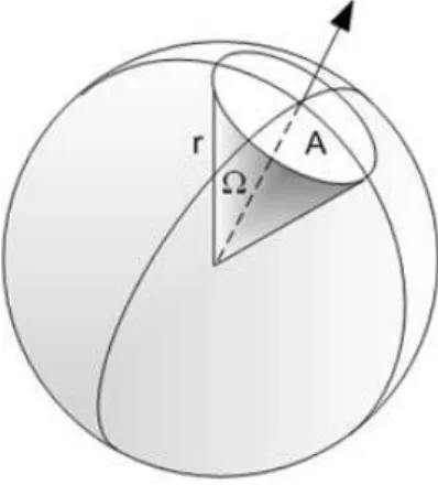
Figure 2.1: Representation of 1 steradian solid angle on a sphere(Fundamentals of Light-ing, 2016).

Ω₌ S

r2, (2.1)

where:

Ω_{is the solid angle (}_sr_);

S is the area (m2);

r is the sphere radius (m).

2.1.1 Luminous Flux

Luminous flux (Φ_V_{) is energy per unit time that is radiated from a source in all directions} over visible wavelengths. The unit of luminous flux is lumen (lm). One lumen is the luminous flux of a uniform point light source that has luminous intensity of 1 candela and is contained in 1 steradian (Figure 2.2). The luminous flux is calculate according to equation 2.2.

Q_V =Φ_V ×_t, _(2.2)

where:

Q_V is the luminous energy (lm.s); Φ_V _{is the luminous flux (}_lm_);

t is the time interval.

(23)

2 . 1 . BA S I C P H O T O M E T R I C P R I N C I P L E S

Figure 2.2: Luminous flux of 1 lumen emitted by a light source (Wikipédia, 2016).

2.1.2 Luminous Intensity

Luminous intensity (I_V) is the amount of visible light emitted by a light source per unit solid angle (Equation 2.3), measured in candelas or lumen per steradian (cd or lm/sr). Luminous intensity is the fundamental SI quantity for photometry and the candela is the fundamental unit from which all other photometric units are derived.

IV = Φ_V

Ω , (2.3)

where:

IV is the luminous intensity (cdorlm/sr); Φ_V _{is the luminous flux (}_lm_);

Ω_{is the solid angle (}_sr_).

2.1.3 Illuminance

Illuminance (E_V) is a measure of photometric flux per unit area (Equation 2.4), or visible flux density. It is a measure of how much the incident light illuminates the surface. A 1 candela light source emits 1 lumen per steradian in all directions. As explained in section 2.1 one steradian has the projected area of 1 square meter at the distance of 1 meter. Therefore, a 1 candela (1cd) light source produces a illuminance of 1 lumen per square meter at a distance of 1 meter. Note that, as the luminous flux projects farther, it becomes less dense, and the illuminance decreases (Figure 2.3).

EV = Φ_V

S , (2.4)

where:

(24)

1 Candela Light Source

1 meter

D meters

E = I/D_V 2 E = 1 lux_V

Figure 2.3: Illuminance.

To reach visual comfort certain levels of illuminance are required, which depend on the tasks developed in the working-spaces. These levels are recommended in the European Standard [22]. Despite it being directed to artificial lighting, it is commonly used to natural lighting since there is no standard in that field available for Portugal.

2.1.4 Luminance

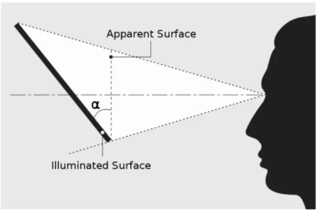
Luminance (L_V) is a measure for the amount of visible light emitted from a surface in a particular direction. It’s the measurable quantity that most resembles a person’s percep-tion of brightness, although they are not really the same. In another words, it’s luminous intensity that emanates from a surface, through it’s apparent surface (Equation 2.5, Fig-ure 2.4). Luminance it’s measFig-ured in candela per square meter or lumen per square meter per steradian(cd/m2orlm/m2/sr).

L_V = IV

S∗cos(_α), (2.5)

where:

EV is the luminance (cd/m2orlm/m2/sr);

IV is the luminous intensity (cdorlm/sr);

S is the projected area (m2);

α is the angle between the illuminated surface and the apparent surface. (m2).

(25)

2 . 2 . S O L A R G E O M E T RY

Figure 2.4: Angle formed by apparent surface and illuminated surface (Adapted from Osram, 2000).

2.2 Solar Geometry

Knowing the sun path is an import information to evaluate the eff_{ect of the sun in} build-ings, either to minimize it’s impacts during the cooling season, or to maximize solar heat gains during the heating season or even to maximize visual comfort inside buildings. In this section the fundamentals to calculate the sun position for a specific time-step at a given location are presented.

2.2.1 Time Definition

There are several ways of expressing the current time in one location, namelysolar time,

local timeandstandard time, the first one is the time used in all of the sun-angle relation-ships.

• Solar timeorlocal solar time (LST) is based on the apparent angular motion of the sun across the sky, with solar noon being the time the sun crosses the meridian of the observer;

• Local time (LT)is based on the diff_{erence between the longitude of the meridian of} a specific local and the longitude of the reference meridian (Greenwich), taking into account that each degree corresponds to 4 minutes addition if east of the reference meridian or subtraction if west of the reference meridian;

• Standard time (ST): as it would not be convenient to have a diff_{erent time for every} place, specific standard times are adopted depending on the time zone where a given place is located.

(26)

a correction from the equation of time is applied. The equation of time expresses the diff_{erence of the solar noon and the time zone noon, which varies with the period of the} year. Equation 2.7 and figure 2.5 express the equation of time.

LST =ST+Lst−Lloc

15 +

E

60, (2.6)

where:

LST is the local solar time;

ST is the standard time;

Lstis the time zone standard longitude;

L_locis the local longitude;

Eis given by the equation of time (equation 2.7).

E= 9,87 sin(2B)−7_,53 cos(_B)−1_,5 sin(_B)_, (2.7) where:

Eis the diff_{erence of the solar noon and the time zone noon in minutes (}_min_);

Bis obtained from the equation 2.8, which depends only the number of the day consid-ered, so 1≤_n≥365.

B= 360×n−81

364 (2.8)

Figure 2.5: Equation of time.

2.2.2 Direction of Beam Radiation

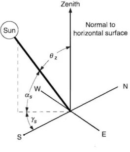
The geometric relationships between a plane of any particular orientation relative to the earth at any time (whether that plane is fixed or moving relative to the earth) and the incoming beam solar radiation, that is, the position of the sun relative to that plane, can be described in terms of several angles [23]. Figure 2.6 represents some of those angles.

The angular position of the sun at solar noon with respect to the plane of the equator, is called declination(δ), varies from−₂₃_,₄₅◦ _{to 23}_,₄₅◦ _{and can be calculated with the} equation 2.9 and its variation is represented in figure 2.7.

(27)

2 . 2 . S O L A R G E O M E T RY

Figure 2.6: Zenith angle (θ_z), solar altitude (α_s) and solar azimuth (γ_s).

sinδ=−sin 23,45 cos360

×₍_n_{+ 10)}

365,25 , (2.9)

wherenis the number of the day considered.

Figure 2.7: Declination variation during the year.

In any place at the surface of the earth, the sun’s rays form an angle with the surface’s normal in that point, that angle is calledzenith angle(θz), which the value can be obtained through the equation 2.10 .

cosθz= cosλcosδcosω+ sinλsinδ, (2.10) where:

θz is the zenith angle (deg);

(28)

δis the declination angle (deg) ;

ωis the hour angle given by the equation 2.11(deg).

ω=(LST−12)×360

24 (2.11)

Frequently, instead of the zenith angle the solar altitude (αs) in used, which is its complementary angle given by the equation bellow.

αs= 90◦−θz (2.12)

The angular displacement from south of the projection of beam radiation on the hori-zontal plane is thesolar azimuth angle(γs), obtained by the equation 2.13. Displacements east of south are negative and west of south are positive.

sinγs=

cosδsinω

sinθ_z (2.13)

An import angle useful for the calculation of shading is theprofile angle(αp), which is the projection of the solar altitude angle on a vertical plane perpendicular to the plane in question, and is given by the equation bellow.

tanαp=

tanαs

cos(γ_s−_γ, (2.14)

where:

αp is the profile angle (deg);

αsis the solar altitude angle (deg);

γsis the solar azimuth angle (deg);

γ is the surface azimuth angle (deg).

2.3 Sky Models

The need for specific and accurate input data for building energy simulation models has become crucial as the users’ needs have become more demanding and the modelling techniques more sophisticated. This is particularly true for the simulation of solar heat gain and daylight availability [24]. For instance, the simulation of daylight distribution in complex interior spaces, requires an accurate knowledge of the distribution of light in the sky [25]. Although sky conditions are constantly changing, typically average sky conditions are used for daylighting simulations. Diff_{erent models of virtual skies have} been developed bye theCommission Internationale d’Éclairage (CIE) and others. In this section two standard sky models developed by the CIE and the Perezet al.sky model are presented.

(29)

2 . 3 . S K Y M O D E L S

2.3.1 CIE Standard Skies

CIE has mathematically developed 15 diff_{erent sky conditions, two of which are shown in} Figure 2.8. Among these sky conditions, overcast and clear skies have been widely used in daylighting simulations all over the world [26].

(a) CIE clear sky (b) CIE overcast sky

Figure 2.8: CIE Sky conditions [26]

• CIE clear sky

A CIE clear sky is defined as having less than 30% of clouds covering the sky or no clouds [26]. It varies according to the altitude and azimuth of the sun, is brighter when closer to the sun and attenuates when moving away from it [27]. Direct sunlight can be considered and calculated inside a build, what makes this model very useful when performing visual glare and thermal discomfort studies.

• CIE overcast sky

This sky model has been widely used when measuring daylight factors, it considers a sky completely covered by clouds and the view of the sun completely impeded (100% covered). Under overcast sky conditions, there is little to no direct lighting and the values of global and diff_{use illuminance are very close [27]. This sky model} is used by designer and users as the worst case scenario.

2.3.2 Perez Sky Model

(30)

The model consists of two independent models:

• Theluminous efficacymodel calculates the mean luminous effi_{cacy of the di}ff_{use and} direct sunlight for a considered sky condition. Input parameters are the solar zenith angle, solar altitude, direct and diff_{use illuminances as well as the atmospheric} precipitable water content [29].

• Thesky luminous distributionmodel yields the sky luminous distribution based on date, time, direct and diff_{use illuminances. The model comprises five parameters} which influence the darkening or brightening of the horizon, the luminance gradient near the horizon, the relative intensity of the circumsolar region, the width of the circumsolar region and the relative intensity of light back-scattered from the earth’s surface [29].

For very dark or bright sky conditions the Perez sky model reduces to the CIE overcast or clear sky [29].

2.4 Daylighting Performance Metrics

2.4.1 Static Daylight Performance metrics

In this section two traditional daylight performance metrics are presented.

2.4.1.1 Daylight Factor

Daylight Factor is defined as the ratio of the internal illuminance at a point in a building to the unshaded, external horizontal illuminance under a CIE overcast sky [30]. Using an illuminance ratio to quantify the amount of daylight in buildings is a concept that has been around for more than a 100 years, in 1909 Waldran has published a measurement technique base on that aproach [31]. The original motive to use ratios instead of absolute values was to avoid the diffi_{culty of dealing with "frequent and often severe fluctuations} in the intensity of daylight" [32]. In it’s early days illuminance ratios were primarily used as legal evidence in court [33], "legal rights of light...constituted practically the only profitable...field for daylight experts" [32]. The UK Prescription Act of 1832 stated that if one has benefited from daylight access across someone’s property for over 20 years an absolute and indefensible right is granted to the window [33]. By analysing these historical facts, it’s plausible to say that measuring the daylight factor was never meant to be for design purposes, but to establish a minimum legal lighting requirement, so it’s use for good design practices seem unfounded.

What is considered to be adequate daylighting levels for various tasks has always been a very important issue. Nowadays 500 lux at work plan is considered to be an adequate

(31)

2 . 4 . DAY L I G H T I N G P E R F O R M A N C E M E T R I C S

level of illuminance for offi_{ce work [22]. Under an overcast sky, 10000 lux can be assumed} for outside illuminance, these corresponds to a daylight factor of 2%.

Daylight factor optimized buildings admit as much daylight as possible, promoting athe more the betterapproach. Taking this into account, a building with a fully glazed envelope is the extreme daylight factor optimized building, yet fully glazed façades are known for having comfort and energy effi_{ciency problems, what makes the above} argu-ment flawed.

Daylight factor has the advantage of having intuitive predictions that are easily com-municated within a design team. On the other hand, daylight factor fails to give a warning flag as to whether certain parts of the building are going to have glare problems or not, in fact it doesn’t even considers the façade orientation, so for east and west facing façades, that are known for having severe glare problems due to being exposed to low solar alti-tudes, it will not be able to help in the development of glare control strategies.

2.4.1.2 View to the outside

A view to the outside is a highly praised benefit of a window by the offi_{ce occupants.} Windows with movable shading devices that are frequently fully lowered to avoid glare problems tend to block outside views, diminishing the benefits of the outside view pro-vided by the window. The view to the outside performance metric is a percentage of working hours when the shades remain open, in the case of a shade half closed, a partial credit is attributed to that time step. For example, in a window with 1m high, and the shade closed 0.2m, a 0.8 value is attributed to the outside view performance metric for that time-step.

2.4.2 Dynamic Daylight Performance Metrics

Dynamic daylight performance metrics were designed to aid the interpretation of climate-based analyses of daylight illuminance levels that are founded on hourly meteorological data for a full year. In opposition to the conventional daylight factor approach, a climate-based analysis employs realistic, time varying sky and sun conditions and predicts hourly levels of absolute daylight illuminance [34]. In the following section several dynamic daylight performance metrics are described.

2.4.2.1 Daylight Autonomy (DA)

(32)

big potential to reduce the needs for electric lighting, and secondly, it doesn’t account the amount by which the threshold was exceed in a particular time step. For offi_{ce spaces the} minimum illuminance required at work plane is 500 lux [22].

2.4.2.2 Continuous Daylight Autonomy (DAcon) and Maximum Daylight Autonomy (DAmax)

This metrics were proposed to tackle the limitations of Daylight Autonomy. Continuous Daylight Autonomy attributes partial credit to time steps when the daylight autonomy fails to reach the minimum daylight illuminance level, instead of focusing on a hard threshold [33]. For example, in a situation where 500 lux are required and only 300 lux are provided by daylight alone, a partial credit of 300lx/500lx = 0.6 is attributed to that time step. The result is that instead of a hard threshold the transition between compliance and non compliance is softened, essentially, this metric acknowledges that even a partial contribution of daylight to illuminate a space is still beneficial [33].

Maximum Daylight Autonomy considers the possibility of glare appearance, it in-dicates the percentage of the occupied hours when direct sunlight or exceedingly high daylight conditions are present, it was defined that the threshold for DAmax is ten times the design illuminance for a given space. In this case study this threshold is 5000 lux.

2.4.2.3 Useful Daylight Illuminances (UDI)

Useful daylight illuminances is also based on the work plane illuminance, but instead of focusing on reaching a defined threshold it aims to determine how often daylight illumi-nances within a range are achieved. This range is defined having illuminance conditions neither to dark (<100 lux) or to bright (>2000 lux) [33], based on this thresholds UDI results in three metrics, which are the percentage of working hours when UDI:

• Was achieved (100 lux-2000 lux);

• Fell-short (<100 lux);

• Was exceeded (>2000 lux).

(33)

C

h

a

p

t

e

r

3

M e t h o d

In the first section of this chapter the simulation process used to obtain the illuminance at work plan and energy consumption values is explained, it starts with a small description of the simulation engines used and then the methodology employed to carry out the computer simulations is explained. The second section of the chapter describes the case study of the research. Finally, the automated control strategies applied to the interior roller shades are described, as well as the simulation results obtained for them.

3.1 Simulation Process

Today there are many simulations tools used to assess the performance of shading devices and evaluate their contribution to the building’s overall energy performance during it’s life circle. Many tools have been used by scientific researchers, engineers and architects to analyse, designate and evaluate daylight values, natural ventilation, indoor thermal and visual comfort. Companies have been developing simulation software, both to assess energy performance of buildings and helping designers predicts real life performance. The use of these programs has increased since the "net-zero energy building" concept became Energy Effi_{ciency Directive [19]. According to a recent study [19], the two most} widely used simulation tools are EnergyPlus and Radiance.

3.1.1 Simulation Tools

(34)

C H A P T E R 3 . M E T H O D

3.1.1.1 Radiance

Radiance is an open source, suite of tools developed to model and visualize the luminous eff_{ects of daylighting systems [36] first created by the}Building Energy Technologies

Divi-sion of Lawrence Berkeley National Laboratoryin Berkeley, California. It uses backward ray tracing and the sky model developed by Perezet al.[28], making possible the simulation of illuminances under any sky condition. Prior to the implementation of daylight coeffi -cient method in Radiance there were few practical options available that enabled annual daylight simulations [37].

The backwards ray tracing method, extends from the original algorithm introduced to computer graphics by Whited in 1980 [38]. Light is followed along geometric rays from the point of measurement into the scene and back to the light sources. The result is mathematically equivalent to following light forward, but the process is generally more effi_{cient because most of the light leaving a source never reaches the point of interest.}

3.1.1.2 EnergyPlus

EnergyPlus is a whole building simulation software used to do energy analysis and ther-mal load simulations. EnergyPlus is the result of the merger ofBLASTandDOE-2 devel-oped by: U.S. Army Construction Engineering Research Laboratories,University of Illinois,

Lawrence Berkeley National Laboratory, Oklahoma State University, GARD Analyticsand

Department of Energy.

The software estimates energy demand considering heat balance between the build-ing interior and the exterior, based on weather information and the characterization of the building, taking into account geometry, construction solutions, thermal loads, air treatment systems, ventilation and occupation patterns [39].

3.1.2 Methodology

The two simulation engines described in the previous section were used to carry out annual dynamic simulations. Firstly, Radiance was used to simulate accurate illuminance values on the work-plane, and secondly EnergyPlus was used to estimate total annual lighting, heating and cooling energy demand. As these two simulation engines aren’t ready to interact with each other, a programming language (Python) was used to create a link between them.

In [40] and [41] Klems proposed a new method to model solar gains through windows with Complex Fenestration Systems (CFS). This method relies on bidirectional optical measurements of CFS to determine reflected and transmitted light by direction for all incident directions defined by the hemisphere viewed by the window, termed bidirec-tional scattering distribution functions (BSDF). Klems also described a means to derive a BSDF for a window system consisting of multiple heterogeneous parallel layers by matrix multiplying the BSDF for each layer, Klems devised a coordinate system that simplified

(35)

3 . 1 . S I M U L AT I O N P R O C E S S

this matrix multiplication. The coordinate system has 145 input and output directions in nine theta bands. The number of phi divisions in each theta band is modulated so that all divisions have roughly the same cosine-weighted solid angle. This BSDF coordinate sys-tem is commonly called the Klems full angle basis. With this BSDF, one can derive total window solar gains via a matrix multiplication of the BSDF coeffi_{cients with incident flux} in each of the 145 window directions, eff_{ectively integrating over the hemisphere seen by} the window [37].

The three-phase simulation method was used in radiance to carry out entire year dynamic simulations of the fenestration systems, and obtain illuminance values at work-plan. This simulation method is based on the daylight coeffi_{cient approach and, it} sepa-rates the light transport between the 145 sky patches defined by Klems and the illumi-nance sensor points into three phases: exterior transport, fenestration transmission and interior transport. Each phase of light transport is simulated independently and stored in a matrix form (Figures 3.1 and 3.2). To obtain the resultant illumination a matrix multiplication is used (Equation 3.1).

i=V T Ds (3.1)

Where,V is a view matrix that relates light from outgoing directions on window to de-sired results at an interior point,T is a transmission matrix that relates incident window directions to exiting directions (BTDF), andDis a daylight matrix that relates the lumi-nance of sky patches to the incident directions on window. By multiplying these three matrices a daylight coeffi_{cient matrix is obtained which is then multiplied by the vector}_s that contains the average luminance of the sky patches for given time and sky conditions.

Figure 3.1: Light transport scheme for the three-phase method.

(36)

Figure 3.2: Radiance three-phase method flow chart [37].

In this study the transmission matrices used were computed using LBNL Window software, which has a large data base of glass types and shading devices, the V matrix containing the two working plane illuminance "sensors" was generated for the offi_ce studied, the D matrix was created using the Radiancertcontribtool, and the s vector was created using a Perez sky model for every hour of the year and TMY data with hourly time steps. Also the parameters passed through Radiance are presented in table 3.1. The three-phase simulation method using these parameters was validated by McNeil et al. in [37].

Table 3.1: Radiance Parameters used in Simulations

Radiance Simulation Parameters V Matrix (Sensor Points) D Matrix

ambient bounces (-ab) 12 4

ambiente divisions (-ad) 60000 2000

ambient subdivisions (-as) 0 0

ambient accuracy (-aa) 0 0

limit weight (-lw) 1e-42 1e-8

direct source subdivisions (-ds) 0,05

-direct jitter (-dj) 1

-direct threshold (-dt) 0

-direct certainty (-dc) 1

-After running the Radiance simulations, Python scripting was used to analyse the resulting illuminance data and create schedules for the artificial lighting power and inte-rior roller shade position, according to the the diff_{erent control strategies applied to them} which, are described in the section 3.3.

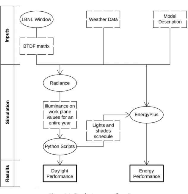
EnergyPlus was then used to estimate total annual lighting, heating and cooling en-ergy consumption. As this simulation engine isn’t prepared to simulate situations where the shades are just partially closed, the window geometry had to be discretized in 20 parts so the interior roller shade is prepared to close in steps of 5%. In figure 3.3 the overall flow chart of a simulation id presented.

(37)

3 . 2 . CA S E S T U DY

Figure 3.3: Simulation process flow chart.

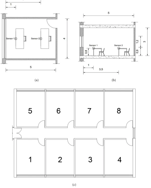
3.2 Case Study

The case study is an offi_{ce room in the middle floor of a building from Faculty of Science} and Technology – Universisdade Nova de Lisboa located in the Lisbon area with latitude = 38.66oand longitude =−9.21o. The space dimensions of the office used in the simulations are 4.0mx 5.0mx 3.0mhigh (represented in figures 3.4(a) and (b) which corresponds offi_{ce number 6 in figure 3.4(c)), with interior surface reflectances for the walls, ceiling} and floor of 50%, 80% and 45% respectively. On its exterior wall the offi_{ce has a window} facing east with 4.0mx 1.2mhigh, which corresponds to a WWR (window to wall ratio) of 40%. The window framing, with a U-value of 1.2W /m2K, accounts for 12% of the total window area. The transparent part of the window is a double clear glazing system with visible and solar transmittances of 0.728 and 0.352 respectively and a U-value of 1.4

(38)

(a) (b)

(c)

Figure 3.4: The image shows the: a) Building floor-plan, b) Offi_{ce used in the case study} floor-plan and c) Offi_{ce used in the case study section.}

The interior roller shade has a solar transmittance of 12%, a solar reflectance of 26% and a visible transmittance of 10%. The fabric used in the roller shade has the same optical properties on both sides.

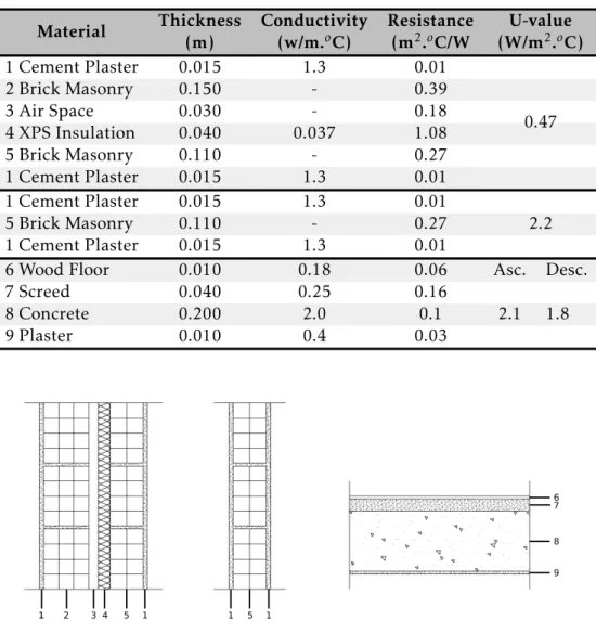
The opaque part of the exterior façade consists in a wall coated on both sides with a cement plaster with 0.015 m, two brick masonry layers, the outer one with 0.15mand the inner one with 0.11m, separated by an air gap of 0.07mpartially filled with thermal

(39)

3 . 2 . CA S E S T U DY

Table 3.2: Glazing optical properties

Visible Solar Transm. Reflect. (Front) Reflect. (Back) Transm. Reflect. (Front) Reflect. (Back) Double Clear

Glazing 0.728 0.098 0.106 0.352 0.301 0.372

insulation of 0.04m which grant’s it a U-value of 0.47W /m2K. The interior walls are made of a brick masonry layer coated on both sides by a cement plaster. The floor and ceiling slabs consist of a concrete layer of 0.20m, a screed of 0.04m, covered on the upper side by a wooden floor of 0.01mand on the down side a plaster of 0.015m(Table 3.3).

Table 3.3: U-value of construction solution.

Material Thickness

(m)

Conductivity (w/m.oC)

Resistance (m2.oC/W

U-value (W/m2.oC)

1 Cement Plaster 0.015 1.3 0.01

2 Brick Masonry 0.150 - 0.39

3 Air Space 0.030 - 0.18

4 XPS Insulation 0.040 0.037 1.08

0.47

2.2

6 Wood Floor 0.010 0.18 0.06 Asc. Desc.

7 Screed 0.040 0.25 0.16

8 Concrete 0.200 2.0 0.1

9 Plaster 0.010 0.4 0.03

2.1 1.8

3 1 1 1

6 9 8 7 5 5 4 2

(40)

Between 8:00 am and 5:00 pm, the offi_{ce is occupied by one person and the electric} equipment load is 5.4 W /m2, which includes only the offi_{ce equipment. The lighting} system is composed by two luminaires with two lamps of 58W each, which produces a power density of 11.6W /m2, continuously dimmable to compensate daylight illuminance, to reach the minimum requirement of 500 lux on the working-plane, which is located 0.8mabove the floor. Heating and cooling is always available throughout the year. The heating set point during offi_{ce hours is 22}o_C _{and 18}o_C _{otherwise, while the cooling set} point is 24oC during offi_{ce hours and 26.6}o_C _{otherwise. Weather data information for} Lisbon was obtained through EnergyPlus Weather website.

Evaluated metrics include a wide range of dynamic daylight performance metrics such as: daylight autonomy (DA), continuous daylight autonomy (DAcon), maximum Daylight Autonomy (DAmax), useful daylight illuminances (UDI) and view to the outside. These metrics were analysed for two diff_{erent points of the work plane, one situated in the front} of the room (sensor 1) and another one in the back (sensor 2). The energy performance metrics presented on this work are: annual energy consumption for lighting, heating and cooling as well as the total energy consumption per unit floor area.

3.3 Shading Control Strategies

In this section the shading control strategies applied to the interior roller shades are presented. Also the results obtained on the simulations are presented and analysed. Automated control strategies similar to the ones used in this study can be found in [18].

3.3.1 No Shading Control

Always open, or without roller shades, and always closed roller shade conditions were first studied as two extreme shading control strategies to provide boundaries for the automated control strategies.

The results provided in table 3.4 show that having no interior roller shades allows a significant amount of daylight into the room, which is equivalent to 96.5% daylight autonomy. It also causes glare problems for a large amount of time, 56.0% of the working hours the illuminance at work plane exceeds 2000 lux. On the other hand, completely closed shades exclude too much daylight from the room resulting in a very low daylight autonomy (9.7%).

In terms of energy consumption, having no interior roller shades is equivalent to almost no need for artificial lighting, while completely closed shades require a constant source or artificial lighting. The total annual energy consumption is 61.5kW h/m2.yearfor roller shades always open, whereas closed shades has an annual energy consumption of 69.6kW h/m2.year, the diff_{erence between the two being caused by the higher amount of} artificial lighting needed in the last case. An unexpected result, was having a lower annual heating energy consumption in the always closed shades situation, when comparing to

(41)

3 . 3 . S H A D I N G C O N T R O L S T R AT E G I E S

the completely open shades, this can be explained by having the lighting system almost always on, which radiates a considerable amount of heat into the room.

Table 3.4: Daylighting and energy performance for the generic case study with the diff er-ent control strategies.

Open Closed CS-I CS-II Sensor Position Number 1 2 1 2 1 2 1 2

Daylight Autonomy (%) 96.5 80.3 9.7 0.1 52.0 26.5 86.5 62.9

Continuous Daylight Autonomy (%) 98.8 92.6 33.3 14.7 71.6 49.6 91.3 80.9

Maximum Daylight Autonomy (%) 25.8 0.4 0.0 0.0 0.0 0.0 12.9 0.0

Useful Daylight Illuminance

not reached (0-100 lux) (%) 0.2 1.0 49.2 80.4 3.7 35.6 4.0 10.3 Useful Daylight Illuminance

(100-500 lux) (%) 3.3 18.7 41.1 19.5 44.2 37.9 9.5 26.8 Useful Daylight Illuminance

exceeded (>2000 lux) (%) 56.0 10.7 0.1 0.0 2.1 0.0 40.7 1.9 Views to the outside (%) 100.0 0.0 45.8 77.8

Annual Lighting Energy

Consumption (kWh/m2_.year) 0.6 10.3 5.9 1.9 Annual Heating Energy

Consumption (kWh/m2_.year) 13.7 11.1 12.5 13.5 Annual Cooling Energy

Consumption (kWh/m2_.year) 47.2 48.1 46.0 44.8 Total Annual Energy

Consumption (kWh/m2_.year) 61.5 69.6 64.3 60.1

3.3.2 Shading Control Strategy I (CS-I)

In order to reduce periods with visual discomfort, in this control strategy, the interior roller shade closes completely when the illuminance at work plane in the front of the room exceeds 2000 lux and direct sunlight is present, as illustrated in figure 3.6. By doing so, the risk of glare occurrence and overheating is reduced, while maintaining good levels of daylighting in the working station which reduce the lighting energy demand. During non-offi_{ce hours the shades are kept closed to reduce solar heat gains during the cooling} season and to prevent heat loss during the heating season. The roller shade position is adapted in hourly time steps.

(42)

Figure 3.6: Schematic view of shading control strategies I, shades close completely when illuminance at work plane exceeds 2000 lux threshold.

also creates long periods with shortage of daylight at the work plane given that daylight autonomy is only achieved in 52% of the working hours.

The total annual energy consumption for CS-I is 64.3 kW h/m2.year which is 4.6% higher than the value corresponding to the completely open shades case. This diff_erence was expected due to higher lighting energy consumption needed (5.9kW h/m2.year) in the presence of a lower daylight autonomy. The heating energy consumption ended up being lower than in the case of the open shades, this can once again be explained by the heat radiating from the lighting system into the room. The annual cooling energy demand was the lowest of the three cases studied at the point, caused by the lower heat gains in the periods when the interior roller shades are closed.

3.3.3 Shading Control Strategy II (CS-II)

The first shading control strategy, CS-I, was based on automatically closing or opening the roller shade depending on the illuminance at work plane value and sun position, to reduce the risk of glare occurrence and overheating. However, this strategy is limited since it only allows fully open or closed positions. In practice, shades might not need to close completely in order to avoid visual discomfort.

Considering this, in the second control strategy, CS-II, the interior roller shades are automatically adjusted to a position that just prevents direct sunlight from falling on the work plane, with hourly time steps, as illustrated in figure 3.7. By doing this, more natural light enters the offi_{ce and thus benefits the occupants. In the present case study} the distance between the roller shade and the work station was set to 1 m as illustrated

(43)

in figure 3.4(b), the determination of the shading position being calculated with the equation 3.2:

LBlind=h−tan(αp)×d (3.2)

where, h is the distance between the working plane and the upper limit of the window, d is the distance between the working area and window andαp is the solar profile angle obtained with equation 2.14.

h

Figure 3.7: Schematic view of shading control strategies II, shades close to a point where they only block direct sunlight from falling on the work-plane.

Shading control strategy II, CS-II, improves daylighting performance significantly, as it lets more natural light in the space by only preventing direct sunlight from falling in the work plane. Although the results for this control strategy show a daylight autonomy of 86.5%, which is 34.5% more than with the control strategy I, it also results in higher percentages of time when the useful daylight autonomy is exceed (40.7%). One of the objectives of this control strategy was to enhance the hours with outside views for the occupants, that objective was reached, as the annual working hours with the shades open are 77.8%, which represents a 32% improvement when compared to CS-I.

The annual cooling energy consumption was the lowest of all four situations (44.8

kW h/m2.year). By having periods with shades partially closed the solar heat gains are controlled while natural light still enters the offi_{ce, reducing the need for artificial} light-ing thus reduclight-ing the heat gains radiatlight-ing from the lightlight-ing system. The total annual energy consumption in CS-II was the lowest of all four cases studied at the point, (60.1

(44)

Despite showing improvement when compared to extreme situation, the automated control strategies where still showing results below expectations. This is due to the optical properties of the glass and roller shade fabric used. In order the enhance daylight and energy performance, in the next section materials with diff_{erent optical properties are} applied to the window.

Figures 3.8 and 3.9 shows the distribution of Daylight Autonomy and percentage of working hours when UDI is exceeded on the working-plane for the generic case study.

Figure 3.8: Daylight Autonomy distribution on work plane for the generic case study and all control strategies.

(45)

(46)

(47)

C

h

a

p

t

e

r

4 I m pa c t o f g l a z i n g a n d s h a d e o p t i c a l

p r o p e rt i e s

The optical properties of the fenestration systems used in buildings have a big impact in daylight and energy performance. Higher solar reflectances block solar radiation from entering the buildings, thus lowering solar heat gains which will reduce cooling energy consumption. While higher visible transmittances will translate in a higher daylight level in the spaces, which will reduce the need for artificial lighting and in turn the lighting energy consumption.

In this section diff_{erent fenestrations systems are presented. Firstly, it is studied the} impact of the interior roller shade fabric optical properties, simulating two additional cases with higher solar reflectance and visible transmittance than the case study already presented. Then the impact of the glazing type optical properties is presented. Once again, two variations of the glazing are simulated, this time with lower solar and visible transmittances than the case study already presented. Finally, the results for all possible combinations between glazing types and interior roller shade fabrics are presented.

4.1 Roller Shade Fabric Optical Properties Impact

(48)

C H A P T E R 4 . I M PAC T O F G L A Z I N G A N D S H A D E O P T I CA L P R O P E R T I E S

solar reflectance to reduce solar heat gains. The optical properties of the interior roller shade fabrics were once again obtained in LBNL Window software and are as follows:

• Roller Shade Fabric II (RSF-II) - solar transmittance of 11%, a solar reflectance of 34% and a visible transmittance of 14%;

• Roller Shade Fabric III(RSF-III) - solar transmittance of 27%, a solar reflectance of 54% and a visible transmittance of 21%.

In all the fabrics used in the roller shades, the optical properties are the same on both sides. An entire analysis was performed for both fabrics described above, and all the results are presented in tables 4.1 and 4.2 and a comparison between them and the generic case is presented in figures 4.1 and 4.2

Table 4.1: Daylighting and energy performance for an offi_{ce with the glazing type I and} roller shade fabric II.

Closed CS-I CS-II

Sensor Position Number 1 2 1 2 1 2

Daylight Autonomy (%) 13.3 0.0 55.6 26.4 86.5 62.4

Continuous Daylight Autonomy (%) 39.7 13.5 76.7 48.9 91.9 80.5

Maximum Daylight Autonomy (%) 0.0 0.0 0.0 0.0 13.2 0.0

not reached (0-100 lux) (%) 28.1 79.8 0.3 35.0 0.2 10.4 Useful Daylight Illuminance

(100-500 lux) (%) 58.5 20.2 44.1 38.6 13.2 27.2

(500-2000 lux) (%) 13.3 0.0 53.6 26.4 45.6 60.5

exceeded (>2000lux) (%) 0.0 0.0 2.0 0.0 40.9 1.9

Views to the Outside (%) 0.0 45.8 77.8

Consumption (kWh/m2_.year) 10.0 5.1 1.9

Annual Heating Energy

Consumption (kWh/m2.year) 11.9 13.3 13.9

Annual Cooling Energy

Total Annual Energy

Despite having higher visible transmittance and solar reflectance, RSF-II haven’t caused a great impact on daylight performance or total annual energy consumption, this is due to small diff_{erences between the optical properties of RSF-I and RSF-II. On the other}

(49)

4 . 1 . R O L L E R S H A D E FA B R I C O P T I CA L P R O P E R T I E S I M PAC T

Table 4.2: Daylighting and energy performance for an offi_{ce with the glazing type I and} roller shade fabric III.

Closed CS-I CS-II

Sensor Position Number 1 2 1 2 1 2

Daylight Autonomy (%) 59.6 11.4 93.7 44.4 94.2 67.8

Continuous Daylight Autonomy (%) 86.4 43.7 98.6 76.4 98.7 85.9

Maximum Daylight Autonomy (%) 0.0 0.0 0.0 0.0 15.5 0.0

not reached (0-100 lux) (%) 2.9 18.2 0.2 1.0 0.2 1.0 Useful Daylight Illuminance

(100-500 lux) (%) 37.5 70.4 6.1 54.7 5.6 31.2

(500-2000 lux) (%) 47.3 11.4 79.4 44.4 50.5 65.9

exceeded (>2000 lux) (%) 12.3 0.0 14.3 0.0 43.7 1.9

Views to the Outside (%) 0.0 45.8 77.8

Consumption (kWh/m2_.year) 4.4 1.7 1.1

Annual Heating Energy

Annual Cooling Energy

Total Annual Energy

hand, RSF-III showed a significant improvement when compared to the other solutions studied either in terms of daylighting or energy performance. For both automated control strategies, SC-I and SC-II, RSF-III was able to reach daylight autonomy values close to the ones obtained in the completely open shade situation, while providing shorter periods when the illuminance at work plan exceeded 2000 lux. When comparing the same shad-ing control strategies between RSF-I and RSF-III, the greater improvement is seen in SC-I, daylight autonomy rises from 52.0% to 93.7%, while the percentage of working hours when UDI is exceeded in the working plan only goes from 2.1% to 12.3%. SC-II reaches a daylight autonomy value of 94.2% but the downside is the UDI exceeded metric, 43.7%. considering this, the highest percentage of working hours when UDI is in the range of 500 lux to 2000 lux, is registered in RSF-III with CS-I, with a value of 79.4%.

In terms of total annual energy consumption, a reduction of 12.9% was observed between the best performing situation in RSF-I (60.1kW h/m2.year) and RSF-III (52.4

(50)

Figure 4.1: Daylight performance for the generic case and the two variations of roller shades fabric.

Figure 4.2: Energy performance for the generic case and the two variations of roller shades fabric.

In the end, the best performing control strategy, both for total annual energy con-sumption and daylighting, became SC-I, while in other situations studied was SC-II.

During the building design process, the decision of which fabric to be used in the roller shade should be made carefully once they can have a significant impact in both daylight performance and total annual energy demand as shown above.

(51)

4 . 2 . G L A Z I N G O P T I CA L P R O P E R T I E S I M PAC T

4.2 Glazing Optical Properties Impact

In this sections instead of changing the roller shades fabric, advanced glazing products were used with the same purpose as in the previous section. Using glass types with lower visible transmittance reduces the amount of daylight which enters the offi_{ce, preventing} work plane illuminance from exceeding 2000 lux, while lower solar transmittance reduces solar heat gains, thus reducing the annual cooling energy consumption.

In addition to the glazing type used in sections 3.2, 3.3 and 4.1, from here on called GT-I (Glazing Type-I), two additional glazing types were modelled and simulated, both with lower solar and visible transmittances then GT-I (Table 4.3).

Once the objective of the research is only to study the impacts of the optical properties of the glass, the U-value of the glazing types used in this section are the same us GT-I. The optical properties of the glazing types were obtained in LBNL Window software and are as follows:

• Glazing type II (GT-II): double glazing with visible transmittance of 0.462 and solar transmittance of 0.248;

• Glazing type III (GT-III): double glazing with visible transmittance of 0.249 and solar transmittance of 0.109.

Table 4.3: Glazing types optical properties

Visible Solar Glazing Type Transm. Reflect. (Front) Reflect. (Back) Transm. Reflect. (Front) Reflect. (Back)

GT-I 0.728 0.098 0.106 0.352 0.301 0.372

GT-II 0.462 0.399 0.294 0.248 0.433 0.465

GT-III 0.249 0.278 0.226 0.109 0.335 0.472

(52)

Table 4.4: Daylighting and energy performance for an offi_{ce with the glazing type II}

exceeded (>2000 lux) (%) 35.0 1.6 0.0 0.0 0.4 0.0 24.4 0.0 Views to the Outside (%) 100.0 0.0 64.0 86.8

Consumption (kWh/m2.year) 52.1 61.5 53.5 50.5

Figure 4.3: Daylight performance for the case study and the two glazing type variations.

(53)

4 . 2 . G L A Z I N G O P T I CA L P R O P E R T I E S I M PAC T

Table 4.5: Daylighting and energy performance for an offi_{ce with the glazing type III}

exceeded (>2000 lux) (%) 23.3 0.2 0.0 0.0 0.1 0.0 10.0 0.0 Views to the Outside (%) 100.0 0.0 76.5 89.0

Consumption (kWh/m2_.year) 46.5 54.6 47.5 45.8

Figure 4.4: Energy performance for the case study and the two glazing type variations.

(54)

roller shade. While, in GT-II and GT-III that diff_{erence was diminished to 2.0% and 1.9%} respectively. In the case of GT-II with shading control strategy II, Daylight Autonomy is 5.2% higher when compared to GT-I with the same control strategy. For control strategy II, the percentage of annual working hours when UDI was exceeded was lower in high quality glazing types, going from 40.7% in GT-I to 24.4% in GT-II, and 10.0% in GT-III. The situation with a higher UDI in the range of 500 lux to 2000 lux was GT-III with CS-II, despite having a lower Daylight autonomy when compared to GT-II with the same control strategy.

Although glazing type II and III showed higher lighting and heating energy demand due to a lower visible and solar transmittance respectively, the opposite occurred in the cooling energy consumption. With lower solar transmittance there was lower solar heat gains which caused a great reduction in cooling energy demand. For the first case studied, GT-I, the higher diff_{erence in the total annual energy consumption was between always} closed shades and shading control strategy II with a diff_{erence of 13.6%. When analysing} GT-II and GT-III the diff_{erence between the same situations became a little higher, 18.0%} and 16.1%. The comparison between the three cases indicates that the glazing type has some impact in the diff_{erent shading control strategies. The shading control strategy} with better energy performance in all three glazing types, showing the lower total annual energy consumption, was SC-II. Using this control strategy in GT-II lead to a total annual energy saving of 16.1%, while in GT-III to 23.8%.

4.3 Final Results Presentation and Discussion

In addition to the fenestrations solutions simulated above, combinations between the glazing types II and III and interior roller shade fabrics II and III where modelled and simulated. The results are presented in this section, as well as an overall comparison of the results of all situations studied. Daylight and energy performance are presented in tables 4.6 and 4.7 respectively, and a comparison between all situations is shown in figures 4.5 and 4.6.

For all three glazing types studied, roller shade fabric II has almost no impact on day-light or energy performance when compared to roller shade fabric I, due to similar optical properties between them. The optical properties of the roller shades fabric have no eff_ect on the percentage of working hours the shades remain open, since the automated shading control strategies rely on the glazing transmitted illuminance alone. When comparing the nine fenestration systems studied, the one with best performance is Glazing Type II combined with roller shade fabric III, using automated control strategy I. Showing one of the highest Daylight Autonomy’s of all combinations studied (92.9%) and a very low percentage of working hours with UDI above 2000 lux (8.8%) thus resulting in the highest percentage of working hours when UDI is in the range of 500 lux to 2000 lux (84.1%). Although, that solution is not the one with the lowest total annual energy demand, it is only outperformed in 2.2 kW h/m2.year (4.6%) by the combination of Glazing Type