Object detection and recognition in complex scenes

UNIVERSIDADE DO ALGARVE

Object Detection and Recognition in

Complex Scenes

Hussein Adnan Mohammed

Master Thesis in Computer Science Engineering

Work done under the supervision of:

Prof. Hans du Buf and Dr. Kasim Terzi´

c

Statement of Originality

Object Detection and Recognition in

Complex Scenes

Statement of authorship: The work presented in this thesis is, to the best of my knowledge and belief, original, except as acknowledged in the text. The material has not been submitted, either in whole or in part, for a degree at this or any other university.

Candidate:

(Hussein Adnan Mohammed)

Copyright c Hussein Adnan Mohammed. A Universidade do Algarve tem o direito, perp´etuo e sem limites geogr´aficos, de arquivar e publicitar este trabalho atrav´es de exemplares impressos reproduzidos em papel ou de forma digital, ou por qualquer outro meio conhecido ou que venha a ser inventado, de o divulgar atrav´es de reposit´orios cient´ıficos e de admitir a sua c´opia e distribui¸c˜ao com objetivos educacionais ou de investiga¸c˜ao, n˜ao comerciais, desde que seja dado cr´edito ao autor e editor.

Abstract

Object Detection and Recognition in Complex Scenes

Contour-based object detection and recognition in complex scenes is one of the most difficult problems in computer vision. Object contours in complex scenes can be fragmented, occluded and deformed. Instances of the same class can have a wide range of variations. Clutter and background edges can provide more than 90% of all image edges. Nevertheless, our biological vision system is able to perform this task effortlessly. On the other hand, the performance of state-of-the-art computer vision algorithms is still limited in terms of both speed and accuracy.

The work in this thesis presents a simple, efficient and biologically moti-vated method for contour-based object detection and recognition in complex scenes. Edge segments are extracted from training and testing images using a simple contour-following algorithm at each pixel. Then a descriptor is cal-culated for each segment using Shape Context, including an offset distance relative to the centre of the object. A Bayesian criterion is used to deter-mine the discriminative power of each segment in a query image by means of a nearest-neighbour lookup, and the most discriminative segments vote for potential bounding boxes. The generated hypotheses are validated using the k nearest-neighbour method in order to eliminate false object detections.

Furthermore, meaningful model segments are extracted by finding edge fragments that appear frequently in training images of the same class. Only 2% of the training segments are employed in the models. These models are used as a second approach to validate the hypotheses, using a distance-based measure distance-based on nearest-neighbour lookups of each segment of the

hypotheses.

A review of shape coding in the visual cortex of primates is provided. The shape-related roles of each region in the ventral pathway of the visual cortex are described. A further step towards a fully biological model for contour-based object detection and recognition is performed by implementing a model for meaningful segment extraction and binding on the basis of two biological principles: proximity and alignment.

Evaluation on a challenging benchmark is performed for both k nearest-neighbour and model-segment validation methods. Recall rates of the pro-posed method are compared to the results of recent state-of-the-art algo-rithms at 0.3 and 0.4 false positive detections per image.

Keywords: object detection, edge fragments, Shape Context, computer vi-sion, human vision

Resumo

Object Detection and Recognition in Complex Scenes

A dete¸c˜ao e o reconhecimento de objetos em cenas complexas, utilizando apenas o contorno ou a forma, ´e um dos problemas mais d´ıficeis na vis˜ao por computador. Muitas vezes, os contornos de objetos s˜ao fragmentados, ocultos ou deformados, e objetos da mesma classe podem ter uma grande varia¸c˜ao. A desordem e as arestas de fundo podem constituir mais do que 90% de todas as arestas de uma imagem. Contudo, o nosso sistema visual ´e capaz de efetuar essa tarefa sem esfor¸co. No outro lado, o desempenho de algoritmos state-of-the-art na vis˜ao por computador ainda fica limitado em termos de velocidade e precis˜ao. As raz˜oes principais, al´em da complexidade das arestas em imagens reais, s˜ao a aplica¸c˜ao de modelos, muitas vezes desenhados `a m˜ao, a aplica¸c˜ao de classificadores complexos, e um longo tempo de treino.

O trabalho nesta tese apresenta um algoritmo simples, eficiente e biologi-camente motivado para a dete¸c˜ao e o reconhecimento de objetos complexos em cenas complexas, utilizando apenas segmentos de arestas dos objetos e dos contornos. Segmentos de arestas s˜ao extraidos das imagens de treino e teste, utilizando um algoritmo simples para seguir arestas ao n´ıvel pixel. Depois, um descritor de cada segmento ´e calculado com o algoritmo Shape Context, inclusive uma distˆancia relativa ao centro do objeto. Basicamente, o algoritmo Shape Context distribui um n´umero de pontos equidistantes, normalmente vinte, sobre um segmento, e um histograma ´e construido para cada ponto. O histograma de cada ponto ´e bidimensional e conta as relac˜oes dos outros pontos em termos de orienta¸c˜oes e distˆancias. Depois, todos os histogramas de um segmento s˜ao concatenados para obter um vetor

des-critivo. Segmentos compridos s˜ao cortados em segmentos menores mas com sobreposi¸c˜oes, para facilitar o processo de emparelhamento entre segmentos em imagens de treino e segmentos em imagens teste.

Um crit´erio Bayesiano ´e utilizado para determinar o fator discrimina-tivo de cada segmento numa imagem teste, aplicando uma pesquisa nearest-neighbour, e os segmentos mais discriminativos de cada classe de objeto votam para potentiais caixas envolventes (limites) de objetos. Depois de eliminar hip´oteses com caixas envolventes sobrepostas, as hip´oteses criadas s˜ao vali-dadas utilizando o algoritmo k nearest-neighbour, com o objetivo de eliminar todas as dete¸c˜oes falsas.

Mais, os segmentos padr˜ao (modelo) t´ıpicos s˜ao extraidos, procurando fragmentos de arestas que aconte¸cem frequentemente nas imagens de treino de cada classe. Apenas 2% dos segmentos de treino s˜ao aplicados nos modelos de objetos. Estes modelos s˜ao utilizados num segundo algoritmo para validar as hip´oteses criadas, utilizando uma medida baseada na distˆancia nearest-neighbour lookup de cada segmento das hip´oteses.

Para atingir um dos objetivos do trabalho, nomeadamente a implementa¸c˜ao de um modelo que ´e ainda mais biol´ogicamente plaus´ıvel, a tese fornece uma revis˜ao da codifica¸c˜ao de formas de objetos no c´ortex visual de primatas. As tarefas ligadas `as formas nas regi˜oes do caminho ventral no c´ortex s˜ao abordadas. Um passo adicional na dire¸c˜ao de um modelo completamente biol´ogico para a dete¸c˜ao e o reconhecimento de objetos, utilizando o con-torno ou a forma, ´e feito pela implementa¸c˜ao de um modelo de extra¸c˜ao de segmentos expressivos e a liga¸c˜ao destes com dois princ´ıpios biol´ogicos: a proximidade e o alinhamento.

A avalia¸c˜ao dos algoritmos desenvolvidos foi realizada utilizando uma benchmark que constitui um desafio, ETHZ, no caso dos m´etodos k

nearest-neighbour e segmentos-modelo de valida¸c˜ao. As taxas recall dos dois algo-ritmis s˜ao comparadas com as taxas de algoritmos do estado da arte recente a dois n´ıveis de fiabilidade: 0,3 e 0,4 dete¸c˜oes positivas falsas por imagem. Embora que os algoritmos desenvolvidos nesta tese s˜ao muito mais simples e r´apidos, os resultados obtidos mostram que ainda n˜ao foi poss´ıvel atingir o topo do estado da arte, mas pelo menos j´a conseguem entrar na competi¸c˜ao.

Termos chave: dete¸c˜ao de objectos, fragmentos de arestas, Shape Context, vis˜ao por computador, vis˜ao humana

Acknowledgements

I would like to express my gratitude to my supervisors Prof. Hans du Buf and Dr. Kasim Terzi´c for the useful comments, remarks and engagement through the learning process of this master thesis. Furthermore, I would like to thank my sister, Sarah, who has supported me throughout the entire process, and my family for their encouragement. Also, I would like to thank the mobility office staff at the University of the Algarve for their constant support.

This work was supported partially by the EU under the FP-7 grant ICT-2009.2.1-270247 NeuralDynamics and the Erasmus Mundus action 2, Lot IIY 2011 scholarship program.

Contents

1 Introduction 1

1.1 General Background . . . 1

1.2 Deep Hierarchy of the Primate Visual Cortex . . . 4

1.3 Challenges . . . 7

1.4 Structure of This Thesis . . . 10

2 Related Work 11 2.1 Object Detection and Recognition . . . 11

2.2 Contour-Based Object Detection and Recognition . . . 14

2.2.1 Computational Methods . . . 14

2.2.2 Biological Models . . . 20

3 Contour-Based Object Detection and Recognition 23 3.1 Feature Extraction . . . 26

3.2 Hypothesis Generation . . . 32

3.3 Validating Hypotheses . . . 34

3.4 Learning Model Segments . . . 36

4 Towards a Fully Biologically Plausible Implementation 41 4.1 Contour Coding in Biological Vision . . . 41 4.1.1 How Does Biological Vision Process Visual Information? 42

4.1.2 How Does Biological Vision Process Shape Information? 44 4.2 Biological Segment Extraction . . . 47

5 Evaluation 52

5.1 Validation on a Standard Dataset . . . 52 5.2 Results . . . 55

6 Discussion and Future Work 63

6.1 Discussion . . . 63 6.2 Future Work . . . 64

List of Figures

1.1 Example of the ability of human vision to detect and recognise objects in a complex scene given only few non-connected edge fragments. . . 2 1.2 Difference between simple and complex scenes. Detecting

ob-jects in complex scenes is no longer a problem of simple shape matching. . . 3 1.3 Two different approaches for shape-based object recognition:

segmentation and edge detection. Images are from the ETHZ dataset [18], see Section 5.1. . . 4 1.4 Simplified hierarchical structure of the primate’s visual

cor-tex and approximate area locations. Box and font sizes are proportional to the area size. Reproduced from [30]. . . 5 1.5 A deep hierarchy versus flat processing scheme. Reproduced

from [30]. . . 7 1.6 Limitation of edge extraction in computer vision. . . 8 1.7 Variation between instances of the same class. . . 8 1.8 Overview of a biologically-inspired active vision system by [66].

The top path models the dorsal pathway (localisation, motion and attention), the bottom path the ventral pathway (recog-nition). Grey text indicates corresponding cortical areas. . . . 10

2.1 Bag-of-Keypoints illustration. Creating histograms from im-age patches. . . 12 2.2 The difference between NBNN and Local NBNN. NBNN forces

a query descriptor di to search for its closest neighbour in all

classes. Local NBNN requires the query descriptor to search only the closest classes. Reproduced from [43]. . . 14 2.3 This is the system proposed by [55]. They proposed an

archi-tecture of the representational and computational system for the detection of 2D shapes. . . 22 3.1 Segment overlapping is necessary to enable many possible matches. 27 3.2 Long contours of objects in complex scenes can be fragmented

into many very short segments. . . 27 3.3 Segment extraction and feature calculation. This is only an

illustration in case of a long contour segment. In reality such long segments are split into overlapping short segments. . . 31 3.4 Different parts of the contour should vote for the same object,

such hypotheses overlaps can be removed easily. . . 33 3.5 False positives can occur during the detection process because

each single segment can generate a hypothesis. None of the hypothesised objects shown here exist in the query image. . . 35 3.6 A single hand-drawn model cannot cope with shape

deforma-tions and intra-class variadeforma-tions. The first and second column show two examples of each class. The third column shows the hand-drawn model of each class as provided in the ETHZ dataset [18]. The fourth column shows model segments for each class as generated by the method proposed in this thesis. The model segments are scaled for better visualisation. . . 39

3.7 Most of the segments inside the bounding boxes of the anno-tated objects belong to clutter or background segments. The first column shows all the extracted segments from the anno-tated objects of the same class. The second column shows the top 50 % of the most frequent segments. The last column shows the top 2% of the segments. Segments are sorted and selected using the method described in the text. The segments are scaled for better visualisation. . . 40 4.1 Illustration of segment merging criteria inspired by

biologi-cal vision. Two constraints are applied: a distance threshold which represents the size of the association receptive field, and orientation difference between nearby segment endings. The green segment (C) should be merged with (A) while the red segments (D and E) are assumed to be not connected. . . 49 4.2 Different modelled cells merge different parts of the contour.

This is useful to provide a description of all possible contour parts. The first column shows an edge map of the object. The second, third and fourth columns show illustration of short edges that can be extracted in the first layers. The fifth column shows contour fragments with specific curvatures. The sixth column shows object parts which result by merging contour fragments from previous layers. . . 50

4.3 A complete shape structure emerges from integrating object parts. The first column shows edge maps of the objects. The second column shows object parts that can be extracted by merging compatible contour fragments similar to the contour fragments recognised in TEO. The third column shows shape structures of entire objects similar to the structures recognised in TE. . . 51 5.1 Examples from the ETHZ dataset [18] which contains five

classes of objects in complex scenes. The first column shows images. The second column shows edge maps of the images. . 54 5.2 Illustration of evaluation metrics for object classification

al-gorithms. A larger intersection area between the green circle (RM or recognition method) and the red circle (GT or ground truth) provides more true positive detections, which means a better performance. . . 55 5.3 Different kinds of curves can be used to visualise the

per-formance of object detection and recognition: ROC and re-call/FPPI curves. . . 56 5.4 Examples of detected objects and their bounding boxes by

using the Bayesian discrimination criterion. The black dots are the centres of the boxes. The first and second column show false positive detections. The third and fourth column show true positive detections. . . 57 5.5 A comparison between the two proposed approaches: using k

Chapter 1

Introduction

1.1

General Background

A distinction is made in the literature between detection and recognition of an object. Detection usually refers to the process of detecting the existence of an object in a given image, together with a rough estimation of the location and size of that object. Recognition is assumed to be the process of identifying and validating detected objects. Recognition can also be considered as a categorisation problem, where the goal is to classify detected objects into certain classes.

Since shape is a natural property of many complex structures, it can be used as a clue to detect and recognise objects, especially when we consider the fact that most objects are best recognised by their global shape, for example bottles and swans.

It has long been known through psychological experiments that shape plays a primary role in real-time recognition of intact objects [5]. In fact, human vision is capable of locating and recognising objects based on their shape easily, even when they are occluded or seen in a heavily cluttered

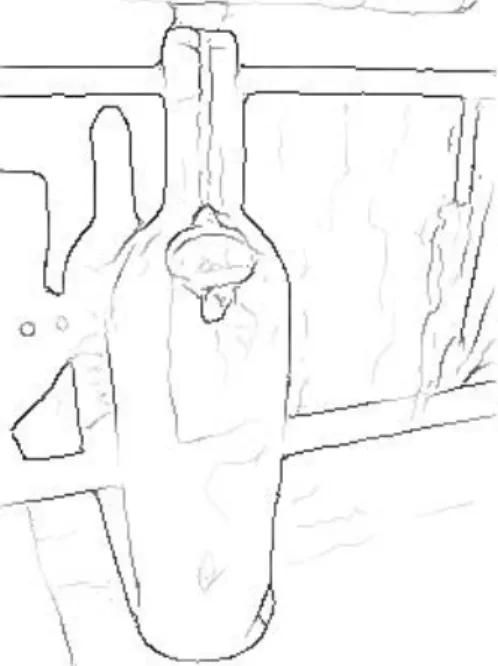
scene. In other words, human vision does not need fully connected contours to recognise objects with distinctive shapes in images; a few non-connected contour fragments are sufficient without any texture or colour information. In Fig. 1.1 we can see an example of the powerful processing capability of the human visual system. We can easily recognise the object given its edge map, despite the missing parts of the contour and the complex background.

Figure 1.1: Example of the ability of human vision to detect and recognise objects in a complex scene given only few non-connected edge fragments.

Shape is perhaps the most important feature in human vision. Conse-quently, it has also been an important field of study in computer vision, artificial intelligence, psychology and cognitive neuroscience. While power-ful computational algorithms exist for recognising complete and clutter-free contours, shape detection in noisy natural images remains a challenging prob-lem. The principal issues are the lack of complete and reliable contours due to the difficulty of bottom-up segmentation, and the presence of occlusions and background clutter.

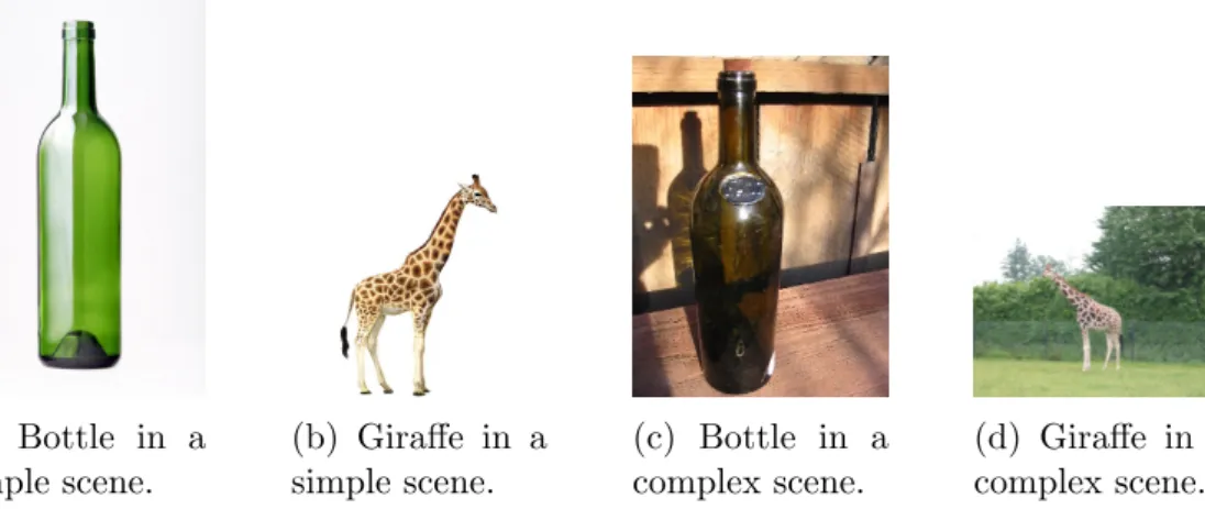
(a) Bottle in a simple scene. (b) Giraffe in a simple scene. (c) Bottle in a complex scene. (d) Giraffe in a complex scene.

Figure 1.2: Difference between simple and complex scenes. Detecting objects in complex scenes is no longer a problem of simple shape matching.

Simple edge fragment descriptors like Shape Context [3] followed by direct distance measurement like the sum of matching errors between corresponding points was enough to recognise and classify clutter-free shapes with complete contours. On the other hand, objects in complex scenes cannot be detected directly by employing their holistic shapes; it is thus no longer a simple shape matching problem. Dealing with fragmented contours where object parts are occluded or connected to clutter is a difficult task indeed, especially if we take into consideration that objects might occupy as little as 10% of the overall image. This means that we have to deal with a very low signal-to-noise ratio; see Fig. 1.2.

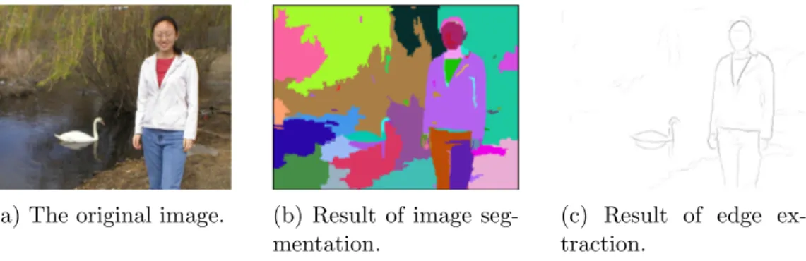
There are two principal approaches to accomplish contour-based object detection and recognition in complex scenes [65]: either by segmenting re-gions, which generally cannot be assumed to correspond to an entire object, or by trying to string together edge segments and corners into complete ob-jects; see Fig 1.3. A comprehensive review of state-of-the-art contour-based object detection approaches can be found in [47]. The edge detection ap-proach is more biologically plausible since experimental evidence and research

(a) The original image. (b) Result of image seg-mentation.

(c) Result of edge ex-traction.

Figure 1.3: Two different approaches for shape-based object recognition: segmentation and edge detection. Images are from the ETHZ dataset [18], see Section 5.1.

suggest that extraction of outermost contours by coding bars and edges in the scene occurs in the visual cortex [48, 58, 5, 11].

The visual cortex in primates is able to accomplish object detection and recognition with an amazing accuracy and in real-time (about 150-200 ms [1]) with almost no effort. Such performance and efficiency has been the goal of computer vision for decades. However, it has never been possible to match human vision’s performance, except on very specific constrained tasks. Nevertheless, much research effort resulted in a rapid increase of the classification rate. In the course of three years, the classification rate on the Caltech-101 database rose from under 20% in 2004 to almost 90% in 2007 [6].

1.2

Deep Hierarchy of the Primate Visual

Cor-tex

Although information about the detailed wiring and functionality is not yet available for most of the regions in the primate visual cortex, the general layout indicates the existence of a deep hierarchy of the different regions with feedback and feedforward connections [30]. This hierarchical system

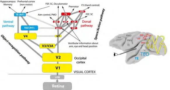
Figure 1.4: Simplified hierarchical structure of the primate’s visual cortex and approximate area locations. Box and font sizes are proportional to the area size. Reproduced from [30].

consists of two interconnected streams: dorsal, which is referred to as the where pathway, and ventral, which is referred to as the what pathway. As the name suggests, the ventral stream (what) is believed to be responsible for object recognition, along with other tasks. A simplified structure of the primate’s visual cortex is illustrated in Fig. 1.4.

In the primary visual cortex, also called area V1, there are simple, com-plex and end-stopped cells. These cells serve to code, at many scales, lines, edges and keypoints. This information is very useful for object recognition. In the hierarchical visual system, simple low-level features are detected and extracted (e.g. orientation, motion, disparity, etc.) over small local regions of visual space in area V1 [53]. These are then combined in higher areas V2 and V4 that have larger visual fields in order to detect more complex and bigger structures like contour fragments, but with a loss of localisation: from local to global representations [11]. These structures are further combined in

the inferior-temporal (IT) cortex to represent even more complex features, which may cover as much as half of the visual field and therefore represent entire objects [58].

It is not yet clear how exactly human vision performs contour-based object recognition. Accumulated evidence suggests that shape representation in primates starts in V4 by recognising meaningful parts of contours, using some kind of curvature calculation on lines and edges extracted in V1 and V2. Then more sophisticated relations are constructed in IT cortex between parts of the same object in accordance with the shape centre to provide the final description of the perceived object in terms of its outermost contours [30].

Due to the complexity of the visual system, most of the current computer vision algorithms avoid implementing such a hierarchy to achieve active real-time vision and focus instead on specific tasks. This approach resulted in flat processing schemes rather than deep hierarchies (see Fig. 1.5), and thus widened the gap between biological and computer vision. Nevertheless, there are some biologically plausible models like HMAX [52], which was extended later in [60], and deep convolutional neural networks (e.g. [29, 8]) which are the result of cumulative efforts since the proposal of the Neocognitron in [20]. These models mimic the hierarchical process in human vision, but they are very slow and resource-demanding, especially during training. The work in this thesis is therefore an attempt to implement a fast and efficient algorithm that is biologically motivated. Although this work is not yet fully biological, it is a first step in this direction.

Figure 1.5: A deep hierarchy versus flat processing scheme. Reproduced from [30].

1.3

Challenges

While we are able to accomplish visual tasks like object detection and recog-nition in complex scenes without any noticeable effort, this is not the case for artificial vision systems. Implementing a fast, efficient and reliable algorithm to do so is a challenging task, knowing that contour-based object detection and recognition in complex scenes has been proven to be one of the most difficult problems in computer vision.

Many problems complicate the ability to detect and recognise an object by its shape within a complex scene (see Fig. 1.6a). Perhaps the worst prob-lem is getting a clean edge map of the scene by low-level image processing. Even with a state-of-the-art edge-detection algorithm, like the Berkeley edge detector [41], we will miss parts of the contours in the presence of clutter; see Fig. 1.6b. In fact, contour extraction has an important top-down com-ponent, and our expectations play a large role to do that. Because of this,

(a) An image of a giraffe in a complex scene.

(b) Edge map of the gi-raffe using the Berkeley edge detector.

(c) The real contours of the giraffe marked man-ually.

Figure 1.6: Limitation of edge extraction in computer vision.

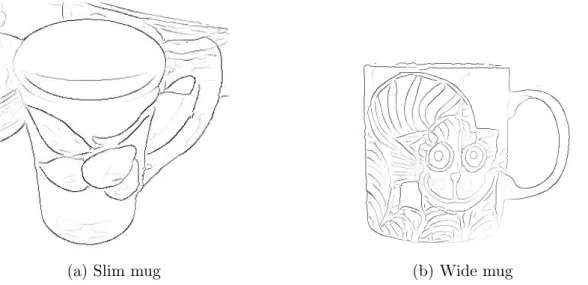
(a) Slim mug (b) Wide mug

Figure 1.7: Variation between instances of the same class.

no purely data-driven, bottom-up algorithm can be expected to extract com-plete object contours; see Fig. 1.6. In addition, objects from the same class can greatly differ, which is referred to as intra-class variation; see Fig. 1.7. Therefore, recognising an object by its shape in a complex scene is not an obvious task at all. In real-world images one can expect all types of compli-cations: clutter, occlusions and intra-class variations, not to mention changes in scale and viewpoint of the objects and scenes.

Furthermore, extracting features locally to obtain global shapes is not possible because shape is an emerging property that becomes only apparent

after all object boundary contours have been grouped, unlike colour or tex-ture which can be captex-tured by small image regions (patches). This leads us to one of two approaches: either connecting fragmented contours depending on some rules like Gestalt principles (proximity, co-linearity, etc.), or try-ing to find some geometrical or spatial relations between fragments. Further details will be provided in Chapter 2.

Despite all challenges that face contour-based object recognition, there is an increasing number of proposed solutions to overcome the obstacles. Nev-ertheless, most state-of-the-art methods are complex and slow (the reasons will be discussed later in Chapter 2), which means that they cannot be used in a real-time scenario. This issue adds an additional challenge: to develop a simple, efficient and fast algorithm.

Developing a biological model for contour-based object recognition can contribute to the unified architecture of active vision as proposed in [66]; see Fig. 1.8. In that work, a number of biologically plausible algorithms are applied in an attempt to build a general-purpose, real-time active vision system. Contour-based object recognition can be integrated as part of the ventral pathway where object recognition takes place.

Recognising an object in early extrastriate cortex (namely area V4) by its shape or even by some of its contour parts is very useful for rapid object categorization. This can trigger attention using fast feedforward (bottom-up) information, such that higher areas like inferior temporal cortex can perform further processing, like biasing likely object categories in memory [59]. This strategy can be helpful in robotics where real-time processing has to be guaranteed: the estimated location of an object in the scene can be passed down from higher areas and it can trigger attention to direct a more precise visual search. Furthermore, contour-based object recognition can be

Figure 1.8: Overview of a biologically-inspired active vision system by [66]. The top path models the dorsal pathway (localisation, motion and attention), the bottom path the ventral pathway (recognition). Grey text indicates corresponding cortical areas.

used as a standalone algorithm in many cases where objects to be recognised are best represented by their shape, such as a traffic environment; see [4].

1.4

Structure of This Thesis

The rest of this thesis is structured as follows: Chapter 2 presents related work in the field of object detection and recognition in general, and in par-ticular the field of contour-based object detection and recognition, the main topic of this thesis. Chapter 3 introduces the developed algorithm to solve the problem of contour-based object detection and recognition in complex scenes. Chapter 4 provides an overview about shape coding and contour-related pro-cessing in the visual cortex of primates and describes a biologically inspired segment extraction approach. Chapter 5 is dedicated to experimental evalu-ation of the methods on a standard dataset. Chapter 6 provides a discussion of presented work and possible future work.

Chapter 2

Related Work

2.1

Object Detection and Recognition

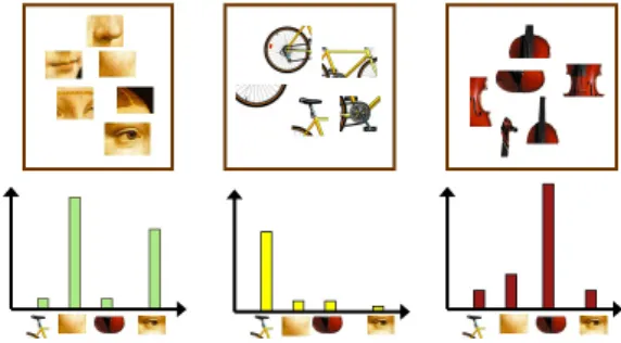
The most common method for object classification in computer vision is Bag-of-Keypoints (BoK) [9]. This method is motivated by the Bag-of-Words (BoW) approach for text categorisation [25, 67, 35]. This technique basically involves the extraction of local features like image patches using any invari-ant descriptor like SIFT [36], then creating a codebook from these features under the independence assumption, e.g., by using k-means clustering and considering each cluster as a word; see Fig. 2.1. Resulting feature vectors are usually classified using powerful parametric classifiers like Support Vector Machines (SVM). Relations between words are not considered in this tech-nique. Since the features are local, spatial information of the patches is not employed. Also, fine differences between features are lost due to the cluster-ing process. Several attempts have been carried out to overcome these weak-nesses. To consider also the spatial layout of extracted features, Lazebnik et al. [31] proposed the famous state-of-the-art Spatial Pyramids technique, which greatly improves the performance of object classification using BoK.

This improvement clearly indicates the importance of considering the neigh-bourhood of extracted features and spatial layout as additional information in object classification.

Figure 2.1: Bag-of-Keypoints illustration. Creating histograms from image patches.

Classification methods can be divided into two categories: parametric and non-parametric. Parametric classifiers construct a model from the data and try to estimate the parameters for that model, while non-parametric classi-fiers attempt to classify by comparing testing data directly with the training data. Each method has its advantages and disadvantages. Obviously, para-metric classifiers require a training phase to determine the parameters of the underlying model. Also, learning a new class typically requires re-training the entire classifier. Furthermore, parametric classifiers are usually resource-hungry and slow during training. On the other hand, the main problem with non-parametric classifiers is poor performance, which has been addressed and fixed by Boiman et al. [6].

Since many non-parametric classifiers are based on nearest-neighbour dis-tance estimation, they inherited the bad reputation regarding low classifica-tion rate that they can offer. This proved to be a wrong assumpclassifica-tion accord-ing to the discussion in [6]. The authors proposed a state-of-the-art classifier which they called Naive Bayes Nearest-Neighbour (NBNN). They argued that two practices actually lead to significant degradation in the performance of

nearest-neighbour distance estimation (and by extension of non-parametric classifiers). The two practices that should be avoided are:

1. Descriptor quantisation: this practice is necessary if we want to construct a codebook for the BoK technique, but it can cause a large loss of information for non-parametric classifiers because they do not have a training phase to compensate this loss. Furthermore, it is not necessary in terms of time efficiency in case of the NN-based technique. 2. Image-to-image distance: measuring the distance between descrip-tors of a query image and descripdescrip-tors of the closest class (image-to-class) directly using nearest-neighbour estimation can provide a much better performance than measuring the distance between descriptors of the query image and descriptors of the closest image (image-to-image), because the search will be generalised to class matching instead of im-age matching and will cope better with intra-class variations.

An NBNN classifier can be summarised as follows:

1. Compute n descriptors d1, ..., dn of the query image q.

2. ∀di ∀c ∈ C compute the NN of di in c: N Nc(di). N Nc is the

Nearest-Neighbour in class c. 3. ˆC = argmin C Pn i=1 k di− N Nc(di) k 2_.

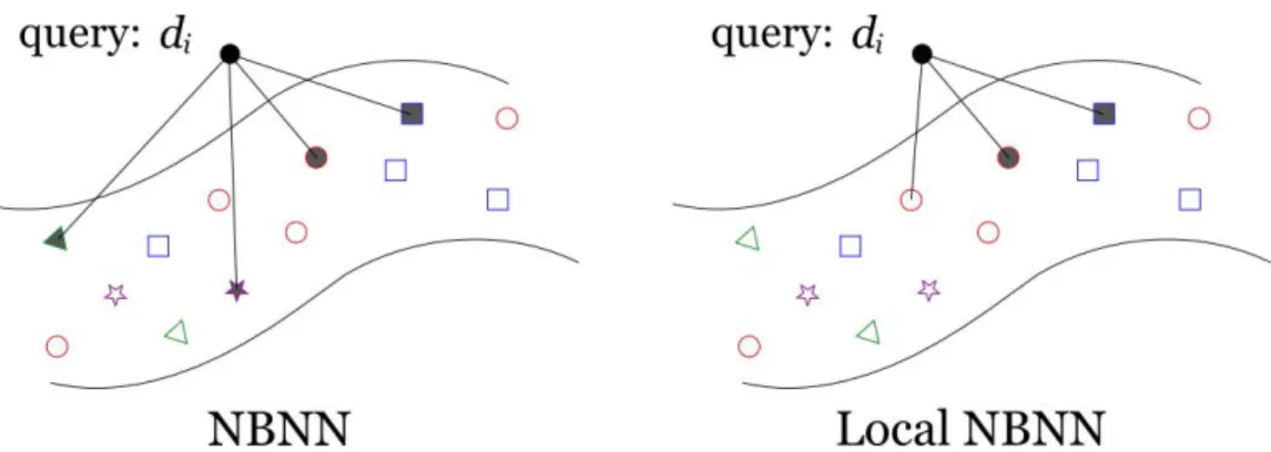
An improvement of NBNN has been proposed in [43], which further in-creased the classification accuracy and improved the ability to scale to a large number of classes (run time of improved NBNN grows with the log of the number of classes rather than linearly); see Fig. 2.2. The main modi-fication is eliminating the need to search for a nearest-neighbour match in

Figure 2.2: The difference between NBNN and Local NBNN. NBNN forces a query descriptor di to search for its closest neighbour in all classes.

Lo-cal NBNN requires the query descriptor to search only the closest classes. Reproduced from [43].

all classes; instead, only the classes within a certain neighbourhood of the query descriptor in feature space are considered. This simple modification results in a significant speed-up over the original NBNN and yields a better performance.

NBNN is typically applied to image patches using descriptors like SIFT in order to classify objects. It has never been applied to contours. The work in this thesis proposes to apply NBNN to contour fragments, as will be shown in detail in Chapter 3.

2.2

Contour-Based Object Detection and

Recog-nition

2.2.1

Computational Methods

In recent years, focus has shifted from classifying entire binarised shapes, where the complete contour of a shape is available, to contour-based object detection in noisy, natural images, such as in the ETHZ Shapes Dataset [18];

see Fig. 1.2. Contours detected in such images are inherently unreliable: objects are typically broken into numerous contour segments, large parts of the object contour may be missing, segments have varying length, and there is a considerable amount of clutter.

Methods for contour-based object detection approach the problem in dif-ferent ways: by using powerful kernel-based classifiers [45, 17], optimised Chamfer matching [34, 61], learning ensembles of short contour segments [50, 19], or by using Gestalt principles for grouping adjacent segments into larger ones [70, 27, 49, 71, 42]. Much of the complexity of these methods is devoted to compensating for incomplete and noisy features.

Many recent state-of-the-art approaches use machine learning algorithms and novel shape models in an attempt to learn consistent configurations and groupings of segments in order to extract reliable features for detection [19, 17, 50, 45]. The steady improvement in detection rates shows that such methods are increasingly successful at extracting information from data, but most of these methods are complex and therefore slow, and knowledge about which segments are useful is often hidden deep inside model parameters.

Several algorithms have been proposed in recent years to perform contour-based object detection and recognition in complex scenes. Although they vary in terms of methodology and structure, they all need a way to de-scribe the features of extracted contour fragments in the edge map of a given image. There exist a number of proposed shape descriptors, but the most common one by far is the Shape Context descriptor [3], which will be de-scribed briefly in Chapter 3. When Shape Context was introduced, focus was on simple closed contour shapes with no scale variations. Attention has shifted since then to recognising objects in complex scenes with intra-class variation in both scale and viewpoint. Since closed contours cannot be

ob-tained in complex scenes, Shape Context can be used to describe individual contour fragments instead of the overall shape; see [75]. Nevertheless, some authors , like Shu and Wu [62], are still investigating global shape descrip-tors inspired by Shape Context to solve simple shape matching with fully connected contours.

After extracting shape features, there is a matching phase between train-ing and query images. A classical method for shape matchtrain-ing is Cham-fer matching, in which the distance is defined as the average distance from points on the training shape to the nearest points on the query shape [2]. However, it has been repeatedly noted that Chamfer matching does not cope well with clutter and shape deformations. Even if a hierarchy of many tem-plates is used to cover deformations, the rate of false positives is rather high (typically more than one false positive per image or FPPI [57]). Neverthe-less, Chamfer matching has not been ignored; [34] improved the accuracy of Chamfer matching while the computational time was reduced from linear to sub-linear. Also, edge orientation information was included in the match-ing algorithm, which resulted in a piecewise smooth cost function. Such improvements allow to use Chamfer matching in the hypothesis validation phase [61].

Fragmented contours in complex scenes can have any length and curva-ture, and they are often caused by clutter in the image. Therefore, some researchers focused on high-curvature points in contours to cope with de-formations of the object, assuming that dede-formations typically happen at high-curvature points. An example is the work done in [50] which uses short line fragments, favouring curved segments over straight ones, and allowing for certain joints by splitting edges at high curvature points. In this thesis we will avoid such “manual” interventions by using a discrimination criterion,

where discriminative segments by definition should have distinctive proper-ties which are specific to the class that the object belongs to.

For category-level object detection, there are two commonly used tech-niques: sliding windows, where windows of different sizes (typically 6-8 sizes) scan the image by moving them a few pixels in each iteration (e.g. [19]), and voting methods which are dominated by the Generalised Hough Transform, where the problem of finding the model’s position in a query image is cast into the problem of finding the transformation parameters which map the model into the image (e.g. [28]). As an alternative to these two leading approaches, [45] proposed a weighted, pairwise clustering of voting lines to obtain globally consistent hypotheses. It is basically a hierarchical approach which is based on a sparse representation of object boundary shape. Then, a verification stage is used to re-rank the hypotheses.

Assuming that contour-based object detection can be formulated as a matching problem between model contour parts and image edge fragments, [72] proposed to solve the problem by finding dominant sets in weighted graphs; the weights are based on shape similarity. Since this approach is based on shape similarity, it can determine an optimal scale of the detected object without the common evaluation of all possible scales. Other work [73] proposed clustering based on the occurrence of patterns of edges instead of visual similarity to create a dictionary of meaningful contours; in other words, contours are matched if they occur similarly in a number of training images.

In an attempt to implement holistic matching of shapes with a large spatial extent, [75] has formulated object detection as a many-to-many frag-ment matching problem by using a contour grouping method to obtain long, salient matching candidates, which are then compared using standard Shape

Context descriptors. The large number of possible matches is handled by encoding the shape descriptors algebraically in a linear form, where optimi-sation is done by linear programming. To evaluate the distance to image segments, they used hand-drawn models.

The idea of explicitly extracting fragments which appear frequently in positive training images of a class, but seldom in negative ones, was explored by Shotton et al. [61]; they learned class-specific boundary fragments and their spatial arrangement as parts of a star-shaped configuration. In addi-tion to their own local shape, such fragments include a pointer to the object centre, enabling object localisation in novel images by using a voting scheme. Also, they employed boosting to select fragments from a large pool of candi-dates. These candidates were constructed by using random rectangles sam-pled from training segmentation masks. The classifier was explicitly trained against clutter to improve the performance. Finally, Chamfer matching was used to validate the hypotheses. The work presented in this thesis shares the idea of selecting fragments that occur frequently in positive training images, but employs a completely different implementation.

Other work has shown that objects can be detected accurately in images using simple model sketches and by building a contour segment network, finding paths that resemble the model chains [18]. Ferrari et al. [18] start by partitioning image edges of the object model into groups of adjacent contour segments. To match these models, they find paths through the segments in the Berkeley edge maps which resemble the outline of the modelled categories. In later work [16], they learned a codebook for Pairs of Adjacent Contours (PAS) directly from cropped training images without any segmented exam-ples and constructed shape models automatically. In order to localise the model in cluttered images, they combined Hough-based centre voting and

non-rigid thin-plate matching techniques. The thin-plate spline model al-lows for a global affine transformation of the shape while also allowing some local deviations from the affine model for each straight contour segment.

To expand their previous research, they presented in [19] a family of scale-invariant local shape features formed by short chains of connected straight contour segments which they call kAS, capable of cleanly encoding fragments of an object boundary. These are then matched to the Berkeley edge map of a query image to detect objects using the sliding window approach. The method offered an attractive compromise between information content and repeatability, and encompassed a wide variety of local shape structures. Fi-nally, they integrated their impressive effort in [17] by learning shape models directly from training images, using only bounding boxes without segmented examples. Then objects are detected and localised at the boundary level, integrating Hough-style voting with a non-rigid point matching (thin-plate spline).

Many recent techniques attempt to segment shapes into visually meaning-ful parts. Although this approach generated impressive results, these tech-niques have only focused on relatively simple shapes, such as those composed of a single object either without holes or with a few simple holes. In many applications, shapes created from images can contain many overlapping ob-jects and holes. Liu et al. [33] proposed a new decomposition method, called Dual-space Decomposition, that handles complex 2D shapes by recognising the importance of holes and classifying them as either topological noise or structurally important.

2.2.2

Biological Models

Inspired by the unmatched level of performance and speed of primate visual systems, researchers have developed computational models to replicate and employ hierarchical process of object recognition in the visual system. Since shape is a primary clue in object recognition [5], several biological models explored the possible representation of shapes, starting from the extraction of simple lines and edges at V1 in early vision to the description of the ob-ject itself using complex relations between contour parts in inferior temporal cortex, and employing intermediate representations of contour parts at V4.

To model line and edge detection in cortical area V1, [53] developed multi-scale models with no free parameters based on responses of simple and complex cells. In [54], the authors emphasised the importance of intermediate 2D shape representation by providing a biologically plausible model which incorporates intermediate layers of visual representation. They proposed that end-stopped and curvature cells are important for shape selectivity.

In a study of the role of area V4 in processing shape information, [48] in-vestigated cell responses to contour features like angles and curves, which are proposed to be intermediate shape primitives by many theorists. Such inves-tigations are important for understanding the transformation from low-level orientation signals to complex object representations. A quantitative model developed in [7] provided a plausible mechanism for shape representation in V4. They considered in their proposed model the selectivity of neurons in area V4 to complex boundary shapes and invariance to spatial translation.

The roles of end-stopping and curvature in intermediate layers of visual representation were modelled in [55]. Shape selectivity in that model is achieved by integrating end-stopped and curvature computations in a hi-erarchical representation of 2D shape; see Fig. 2.3. This model shows the

critical role that end-stopped neurons play in achieving shape selectivity.

The work presented in this thesis is based on nearest-neighbour lookups, which can be done efficiently using the K-D tree implementation provided by the FLANN library [44]. In order to avoid generating a huge number of hy-potheses by using the sliding window technique as used in many algorithms (e.g. [19]), here we will use a Bayesian criterion to determine the discrimina-tive power of each segment in a query image and let the most discriminadiscrimina-tive segments vote for potential bounding boxes. Since closed contours cannot be obtained in complex scenes, Shape Context [3] will be used to describe the individual contour fragments instead of the overall shape. We will avoid man-ual selection of high-curvature points in contours, which is applied by some methods like [50], by using a discrimination criterion, where discriminative segments by definition should have distinctive properties which are specific to the class that the object belongs to. Also, a fast method will be proposed to extract meaningful model segments, by finding edge fragments that appear frequently in positive images of the same class. The same idea was employed by Shotton et al. [61] but with a completely different implementation.

Figure 2.3: This is the system proposed by [55]. They proposed an architec-ture of the representational and computational system for the detection of 2D shapes.

Chapter 3

Contour-Based Object

Detection and Recognition

The work in this chapter is mostly inspired by biological vision in terms of (1) using contour parts with certain curvatures as triggers to drive the attention for a more precise search, (2) using a coding scheme similar to log-polar mapping in V4 to describe shapes of contour fragments, and (3) using the absolute distance from contour fragment to shape centre as impor-tant information that helps relating fragments of the same contour together. In the next chapter, a further step will be taken towards a fully biological implementation.

Two important metrics in the evaluation of object detection and classi-fication algorithms are precision, which is the percentage of the correct de-tections among all generated hypotheses by the algorithm and recall, which is the percentage of correctly detected objects. Most proposed algorithms for object detection and recognition consist of two basic steps: (i) detec-tion, which identifies potential object locations and sets the upper bound on achievable recall; see Eqn. 5.2, and (ii) verification, which eliminates false

positive detections and sets the upper bound on precision; see Eqn. 5.1. Many modern algorithms implement the detection stage by using a sliding window at varying scales, and rely on a powerful binary classifier to eliminate false detections. This approach works well if the binary classifier is accurate, but it also results in slower recognition. In order to avoid that delay, here we will use a Bayesian criterion to determine the discriminative power of each seg-ment in a query image in order to let the most discriminative segseg-ments vote for potential bounding boxes. Also, we try to locate meaningful segments which most likely correspond to object contours.

The work presented in this thesis is based on nearest-neighbour lookups, which can be done efficiently using K-D trees implementation provided by the FLANN library for nearest-neighbour lookups [44]. Recent work in image classification has exploited the fact that conditional class probabilities can be well approximated by the Euclidean distance to the nearest feature belonging to the correct class [6], as shown below.

Given a query image q represented by a set of local features d and a set of classes C, it can be classified as belonging to class c ∈ C according to the conditional probability

c = argmax

C

p(C|q). (3.1)

By applying Bayes’ theorem and assuming a uniform prior probability over classes we obtain

c = argmax

C

p(q|C). (3.2)

If the n descriptors di, extracted from image q, are assumed to be

indepen-dent, the equation can be re-written as

c = argmax C " log( n Y i=1 p(di|C)) # (3.3)

= argmax C " _n X i=1 log p(di|C) # . (3.4)

The probability p(di|C) in Eqn. 3.4 can be approximated using a Parzen

window estimator, with kernel K, i.e.,

ˆ p(di|C) = 1 L L X j=1 K(di− dcj), (3.5)

where L is the number of descriptors that belong to class c in the training set, and dc

j is the j-th nearest descriptor to di in class c. A further approximation

can be done by using only the r nearest-neighbours,

ˆ pr(di|C) = 1 L r X j=1 K(di− dcj). (3.6)

It can be approximated further by considering only the single nearest-neigh-bour (NNc(di)) by setting r to 1:

ˆ

p1(di|C) =

1

LK(di− NNc(di)). (3.7) Substituting Eqn. 3.7 into Eqn. 3.4 and using a Gaussian kernel for K gives

c = argmax C " _n X i=1 log 1 Le − 1 2σ2kdi−NNc(di)k 2 # (3.8) = argmin C " _n X i=1 k di− NNc(di) k2 # , (3.9)

where (log) is the natural logarithm.

The last Eqn. 3.9 shows that conditional class probabilities can be ap-proximated by the Euclidean distance to the nearest feature belonging to the

correct class. In other words, it suffices to find the class with the minimum Euclidean distance of its features to those of the query image.

This approximation performs well as long as there is a large number of training features. Instead of trying to discover meaningful rules for merging and splitting segments, our approach will rely on statistics present in training images to discover meaningful segments.

In a nutshell, the method performs the following steps: (i) extraction of many segments from training and testing images; (ii) for each segment in a test image, find the k nearest-neighbours among training segments; (iii) keep-ing a small percentage of segments after applykeep-ing a Bayesian discrimination criterion; (iv) creating bounding-box hypotheses from each of the selected segments; and (v) classifying the hypotheses as object or background based on k nearest-neighbours.

3.1

Feature Extraction

Contour extraction in natural images is a difficult task. We start with the results of the excellent Berkeley edge detector [40], which are provided as part of the ETHZ dataset [18] and are also used as a starting point by most other algorithms. This is a bottom-up approach, so the extracted edges do not always correspond to object boundaries.

In order to provide sufficient training samples for reliable nearest-neigh-bour lookups, a large number of overlapping segments is extracted to ensure that each segment in a test image can have a close match; see Fig. 3.1. The approach is simple: contour-following at each edge pixel is applied, in order to extract many possible segments of many possible lengths, the pseudo-code for segment extraction is shown in Algorithm 1. Fig. 3.2 demonstrates the

(a) Original seg-ment. (b) First over-lapping sub-seg-ment. (c) Second over-lapping sub-seg-ment. (d) Third over-lapping sub-seg-ment.

Figure 3.1: Segment overlapping is necessary to enable many possible matches.

(a) An image of a giraffe in a complex scene.

(b) Edge segments long-er than 3 pixels.

(c) Edge segments long-er than 100 pixels.

Figure 3.2: Long contours of objects in complex scenes can be fragmented into many very short segments.

importance of short segments in complex scenes. Therefore, after counting the number of pixels of each edge fragment, only fragments with a length of at least 20 pixels are kept because of Shape Context (see below). Larger frag-ments are split into smaller but partially overlapping fragfrag-ments, but always with at least 20 pixels. For example, if a fragment counts 100 pixels, three fragments of 50 pixels are created, at the two ends and in the middle. In case of bifurcations, all possible paths are considered as long as the resulting fragments have at least 20 pixels. During training, only annotated regions containing objects are used.

Algorithm 1 Extraction of all segments starting at a pixel location. input : starting point pt0 = [x0, y0]

output: set of all segments starting with pt0

AllSegments ← [] ActiveSegments ← [] S ← [pt0] ActiveSegments ← [ActiveSegments; S] repeat NextActiveSegments ← [] for S ∈ ActiveSegments do for pt ∈ neighbours(S[last]) do

if pt is an edge pixel and pt /∈ S then S0 ← [S, pt] AllSegments ← [AllSegments; S0] NextActiveSegments ← [NextActiveSegments; S0] end if end for end for ActiveSegments ← NextActiveSegments until ActiveSegments = ∅ return AllSegments

because it ensures that parts of long contours can be matched to short con-tour fragments. Although this method generates a large number of segments, this is not a problem because a discriminative power criterion will be intro-duced later for measuring how meaningful each segment is. In practice, the algorithm works well even with a small subset of segments.

The algorithm presented in this thesis does not attempt to split segments into sections between junctions like in [50], because there are many junctions between object contours and background segments. Also, Gestalt grouping principles are not applied. Instead, the available partial segments are con-sidered as they are and we will try to find the best possible explanation for each of them. We intentionally kept feature extraction simple in order to find out how much information is actually present in the data, before introducing additional knowledge.

For each extracted segment, a feature vector is calculated. This starts by computing the Shape Context parameters [3] based on 20 equidistant points on the segment, and by concatenating them into one long descriptor. After careful experimentation, the following parameters are used: 12 orientation intervals of 30 degrees each, 3 distances that increase logarithmically starting from the point, and a maximum distance that covers 80% of segment length; see Fig 3.3. These parameters give descriptors of 720 bins in total, many bins being empty (zero) of course. Since each segment is sampled using a fixed number of equidistant points, the descriptors are size invariant. Rotation-invariance can be achieved by rotating each segment so that the ending points are aligned to the x-axis before calculating the Shape Context descriptor. We note that rotation-invariance has not been included when validating the method on the ETHZ dataset. Below is the procedure of calculating Shape Context:

1. Select N equally spaced points along the segment (N = 20), including the end points.

2. Calculate the vectors from each selected point pi to the other points

pj6=i.

3. Create a histogram hi of vectors for each point

hi = #{pj 6= pi : (pj − pi) ∈ bin(k)},

where k is the number of bins in the histogram.

4. Concatenate the histograms of all points into one vector for each seg-ment.

The offset from the centre of each segment to the centre of the bounding box in the training image is also added to the descriptor. This offset is used during hypothesis validation because each hypothesis has an estimated centre. During object detection, only Shape Context descriptors are used.

During training, the class of shape (object) which the segment belongs to is recorded. Its centre offsets from the top-left and bottom-right corners of the annotated object bounding box are also recorded. A background class is learned by extracting many segments from outside the bounding boxes of objects in all training images of all object classes. The descriptors of all collected segments are stored in an efficient K-D tree implementation provided by the FLANN library for nearest-neighbour lookups [44].

(a) Edge map of an Apple logo. (b) Extracted segment from the edge map.

(c) Shape Context illustration. 20 equidistant points are distributed over the segment. Each point has a histogram which consists of 12 orien-tations and 3 logarithmic distances.

Figure 3.3: Segment extraction and feature calculation. This is only an illustration in case of a long contour segment. In reality such long segments are split into overlapping short segments.

3.2

Hypothesis Generation

Hypothesis generation also starts by extracting all segments from a test im-age and by calculating their feature vectors, as described in the previous section. Most of the extracted segments typically belong to the background, or do not help much in distinguishing between shapes (such as straight lines). Therefore, a Bayesian discrimination criterion is applied in order to select the most discriminative segments for a class:

Dc(di) :=

P (di | c)

P (di | ¯c)

, (3.10)

where di is a feature descriptor associated with segment Si of class c, and

P (di | ¯c) is the probability that di was generated by any class except c.

The probabilities are estimated using Eqn. 3.9 and an approximate dis-tance measure is obtained:

log Dc(di) ≈ distc(di) − dist¯c(di), (3.11)

where

distc=k di− N Nc(di) k2; dist¯c=k di− min ¯

c6=c N N¯c(di) k 2

.

For each segment extracted from a test image, the nearest neighbours of the training segments are determined in feature space using the FLANN library [44]. Then the class label of the nearest neighbour is assigned to the query segment. The discriminative power of each segment in the test image is calculated using Eqn. 3.11. The segments are then sorted by their discriminative power. Finally the most discriminative segments are kept.

(a) Edge map of an Ap-ple logo image.

(b) First discriminative segment voting for the Apple logo.

(c) Second discrimina-tive segment voting for the Apple logo.

Figure 3.4: Different parts of the contour should vote for the same object, such hypotheses overlaps can be removed easily.

During training, the offset of the central point of each segment from the top-left and bottom-right corners of the bounding box containing the object is stored. During detection, this information is used to create an object hypoth-esis consisting of a bounding box and a class label for each discriminative segment; see Algorithm 2.

A hypothesis which overlaps with another hypothesis of the same class by more than 90% (the area of the intersection of the bounding boxes over the area of the union) is removed to reduce the number of hypotheses without impacting the recall. This can happen because many parts of the contour should vote for the same object, as illustrated in Fig. 3.4. Nevertheless, overlapping segments are needed to guarantee the existence of a segment’s match despite the variation of contour fragments’ lengths in each object instance.

Since each single segment can generate a hypothesis, two restrictions are imposed to eliminate meaningless hypotheses: hypotheses that have less than 50% overlap with the test image are eliminated, which can occur at the image border, and hypotheses with very few segments are assumed to be empty and

ignored. These two restrictions have absolutely no effect on the detection result and significantly reduce the number of generated hypotheses.

The process described above guarantees that segments triggering hy-potheses are discriminative and meaningful, but they can still be false pos-itives because the existence of one part of the contour does not necessarily mean that there is an object; see Fig. 3.5. The detection step results in about 16 hypotheses per class per image on average on the ETHZ dataset, without missing any object, but precision is still bad. The number of generated hy-potheses depends mostly on the number of segments in the image and how many discriminative segments are kept.

Algorithm 2 Hypothesis generation for all classes.

input : all image segments ImgSegments, all training segments TrSeg-ments, all training bounding boxes TrBoxes

output: set of all hypotheses AllHypotheses ← []

for S ∈ ImgSegments do

Neighbours ← kNearestNeighbours(S, TrSegments) NearestSegment ← Neighbours[0]

Class ← class(NearestSegment)

NearestOther ← Neighbours[i], where class(Neighbours[i] 6= Class) Discriminative power ← dist(NearestSegment)2_{− dist(NearestOther)}2

BoundingBox ← TrBoxes(NearestSegment) scaled to match S CurrentHypothesis ← S, Class, BoundingBox, Discriminative power AllHypotheses ← [AllHypotheses; CurrentHypothesis]

end for

GoodHypotheses ← percentage of most discriminative hypotheses return GoodHypotheses

3.3

Validating Hypotheses

The final step of the algorithm is to process all object hypotheses and to try to discard any false positives. For each hypothesis generated in a test image

(a) False positive due to a bottle-like segment corresponding to the right part of a bottle.

(b) False positive due to a giraffe-like segment corresponding to the head of a giraffe.

(c) False positive due to a mug-like segment corresponding to the upper-left part of a mug.

(d) False positive due to a swan-like segment corresponding to the upper part of a swan.

Figure 3.5: False positives can occur during the detection process because each single segment can generate a hypothesis. None of the hypothesised objects shown here exist in the query image.

by the previous step, all segments within the estimated bounding box are selected and the hypothesis is classified as object or background, depending on a simple strength measure.

For each segment selected from the hypothesis, the number of neighbours of training segments in feature space of the same class label given to the hypothesis is counted, as is the number of neighbours of any other class label. The ratio of these two numbers represents the strength value of this hypothesis: Strength-kNNc_h = Pk i=0Nic Pk i=0N ¯ c6=c i . (3.12)

Strength-kNNc_h is the strength measure of hypothesis h of class c, and k is the number of neighbours of each segment. Nc

i is one if the neighbour is of

the same class label of the hypothesis and is zero otherwise. Nc¯

j is zero if the

neighbour is of the same class label of the hypothesis and is one otherwise. All hypotheses which overlap with a stronger hypothesis of the same class by more than 50% (PASCAL criterion) are eliminated, such that only one object of a particular class is allowed to exist at a given position in the image. Finally, all the hypotheses are sorted by decreasing strength. A threshold is applied to the remaining hypotheses, and this threshold is the free parameter of this method which can be used for balancing precision and recall.

3.4

Learning Model Segments

Many researchers use hand-drawn models to estimate kernel parameters for classification (e.g. [45]) or to match them directly to the query images us-ing template matchus-ing techniques like Chamfer Matchus-ing [34, 61]. Such models do not cope well with shape deformations and intra-class variations

because one model cannot represent a whole class in most cases; see Fig. 3.6. Therefore, some authors prefer to learn models directly from training images (e.g. [17]).

Learning shape models from training images is a very complicated and slow part in most state-of-the-art algorithms. Also, these models often do not provide information about important contour parts in each class. A simple, fast and efficient method is proposed here to extract meaningful model seg-ments by finding edge fragseg-ments which appear frequently in positive images of the same class.

Meaningful model segments are extracted from training images using nearest-neighbour lookups. An identification number is assigned to each object in the training images. This identification number is attached to the training segments during the extraction process. After extracting segments from training images as described earlier, the most similar segments are de-termined for each training segment using the FLANN library [44]. Then the number of nearest neighbours in descriptor space with the same class label but from different objects is incremented, until a neighbour with a different class label is found. Finally, training segments are sorted according to their number of neighbours and only the top 2% are used to create the models. This very low percentage of segments indicates the huge amount of clutter inside the bounding boxes of training images and the powerful selectivity of this simple method; see Fig. 3.7.

Since models extracted in this work consist of many individual segments, important parts of object contours can be recognised and learned easily with many possible deformations. These models can be used directly by match-ing model segments to test segments. Each class model consists of the most frequently occurring and most similar segments in the bounding boxes of

training images. Therefore, the sum of distances of test segments of a hy-pothesis to the model segments of the same class can be used as a measure of strength for that hypothesis. These distances are normalised by the number of segments of the hypothesis:

Strength-Modelsc_h = 1 Average-Distancec_h, (3.13) Average-Distancec_h = Pn i=0dist c i n , (3.14)

where n is the number of segments of the hypothesis, distc_i is the distance of the ith segment in the hypothesis of class c to the nearest model segment of the same class and Average-Distancec_h is the average distance of hypothesis h of class c to the model segments of the same class.

Figure 3.6: A single hand-drawn model cannot cope with shape deformations and intra-class variations. The first and second column show two examples of each class. The third column shows the hand-drawn model of each class as provided in the ETHZ dataset [18]. The fourth column shows model segments for each class as generated by the method proposed in this thesis. The model segments are scaled for better visualisation.

Figure 3.7: Most of the segments inside the bounding boxes of the annotated objects belong to clutter or background segments. The first column shows all the extracted segments from the annotated objects of the same class. The second column shows the top 50 % of the most frequent segments. The last column shows the top 2% of the segments. Segments are sorted and selected using the method described in the text. The segments are scaled for better visualisation.

Chapter 4

Towards a Fully Biologically

Plausible Implementation

In the previous chapter, a method mostly motivated by biological vision has been presented to detect and recognise objects by their contour frag-ments. This chapter presents a further step towards a fully biological model of contour-based object detection and recognition in complex scenes.

A general and brief description is provided first about the visual system in primates, followed by an overview about shape coding of fragmented con-tours. Finally, a biologically inspired segment extraction method is proposed.

4.1

Contour Coding in Biological Vision

The work on the cat’s visual cortex by Hubel and Wiesel [24] was an impor-tant motivation for Marr [39] and others to build visual hierarchies analogous to the primate visual system. Such computational modelling of biological vi-sion can serve two goals: first, it provides a better understanding of the detailed wiring and functionality of the visual cortex; second, it gives

in-sight and inspiration for computer vision to build an active vision system that can be used in real-time applications, with the ability of general scene understanding.

4.1.1

How Does Biological Vision Process Visual

In-formation?

Processing visual information in primates starts in the retinae of both eyes, then the signals are gathered in the Lateral Geniculate Nucleus (LGN) for further processing before they enter the visual cortex. This stage is called pre-cortical processing. In the visual cortex, early vision processing starts in the occipital part of the cortex which consists of areas V1-V4 and the middle temporal cortex (MT). Two interconnected streams emerge at this stage of processing: dorsal, which is referred to as the where pathway, and ventral, which is referred to as the what pathway. The ventral stream from V1 to IT is responsible for invariant object recognition. The dorsal stream deals with disparity, motion and attention.

Receptive fields of neurons in visual cortex increase in size gradually from very small spatial regions in V1 and V2 to half of the visual field in areas like TE. These receptive fields are retinotopically organised in early vision areas; in other words, adjacent neurons cover adjacent visual locations.

Such a hierarchical system is able to share information and low-level fea-tures in different visual tasks at the same time. A generic description of visual properties is extracted in areas V1-V4 and MT, which cover about 60% of the size of visual cortex [13]. This fact indicates the importance of general-ity and the concept of using basic perceptual entities as building blocks to perform different visual tasks. Furthermore, the concept of a deep hierarchy is linked to object recognition as neurophysiological evidence suggests [64].

In order to provide learning ability and adaptation to the system, vi-sual representations increase gradually along the way up in the hierarchical structure, starting from the retina where no evidence of learning is observed [21] up to IT cortex where measurable changes even at a single-cell level have been observed due to learning and adaptation [32]. Such plasticity in later areas of the visual cortex allow primates to learn new objects and new representations of the same objects.

In order to pave the path for computer vision, authors in [30] provided a sufficient, and yet simple, description of the visual cortex in primates, so artificial vision’s engineers can learn from and be inspired by the powerful hierarchy in biological vision (see Fig 1.4). The provided guidelines can be summarised as follows:

1. Hierarchical processing can be useful for:

• Computational efficiency: in case of the availability of multiple processing units and GPUs.

• Learning efficiency: because

– Objects and scenes are hierarchical by nature so it will be easier to structure them in terms of their parts.

– Appropriate features at a relatively high level will already be available in case of hierarchical processing.

2. Separation of information channels can be useful for:

• Cases where some information channels are not available at all times.