Fuzzy Inference Systems Composed of Double-Input Rule Modules for Obstacle Avoidance Problems

(1)

Fuzzy Inference Systems Composed of

Double-Input Rule Modules for Obstacle

Avoidance Problems

Hirofumi Miyajima, Takehiro Kawai, Noritaka Shigei, and Hiromi Miyajima

Abstract—The purpose of self-tuning algorithm for fuzzy inference system is to construct automatically fuzzy inference rules from learning data based on the steepest descend method. Obvious drawbacks of the method are its large computational complexity and getting stuck in a shallow local minimum. Further, it is difficult to apply for the conventional method to the problem with a large number of variables. In order to overcome them, the SIRMs (Single-Input Rule Modules) and DIRMs (Double-Input Rule Modules) models have been proposed. In some numerical simulations, it is shown that there exists the difference of the ability between DIRMs and SIRMs models. In this paper, we will apply DIRMs and SIRMs models to the control problem of obstacle avoidance. As a result, it is shown that DIRMs model is more effective than SIRMs model in this problem. Further, we propose a learning method to reduce the number of modules of DIRMs model and show the effectiveness in numerical simulations.

Index Terms—Fuzzy inference model, Single-input rule mod-ule, Small number of input rule modmod-ule, Double input rule module, obstacle avoidance.

I. INTRODUCTION

M

ANY studies on self-tuning fuzzy systems have been made [1], [2]. The aim of these studies is to construct automatically fuzzy inference rules from input and output data based on the steepest descend method. Obvious draw-backs of the method are its large computational complexity and getting stuck in a shallow local minimum. Further, there is a problem that the number of fuzzy rules increases with increasing of input variables [3]–[5]. In order to overcome them, some novel methods have been developed which 1) create fuzzy rules one by one starting from any number of rules [6], 2) delete fuzzy rules one by one starting from a sufficiently large number of rules [7] , 3) use GA and PSO to determine the structure of the fuzzy model [4], [15], 4) use a self-organization or a vector quantization technique to determine the initial assignment of fuzzy rules [8], and 5) use generalized objective functions [9]. However, there are little studies on effective learning methods of fuzzy inference systems dealing with a large number of input variables; in

Manuscript received July 8, 2014

Hirofumi Miyajima is with Graduate School of Science and Engineering, Kagoshima University, 1-21-40 Korimoto, Kagoshima 890-0065, Japan (e-mail: k3768085@kadai.jp).

T. Kawai was with Graduate School of Science and Engineering, Kagoshima University, 1-21-40 Korimoto, Kagoshima 890-0065, Japan (e-mail: k8005442@kadai.jp).

N. Shigei is with Graduate School of Science and Engineering, Kagoshima University, 1-21-40 Korimoto, Kagoshima 890-0065, Japan (e-mail: shigei@eee.kagoshima-u.ac.jp).

Hiromi Miyajima is with Graduate School of Science and Engineering, Kagoshima University, 1-21-40 Korimoto, Kagoshima 890-0065, Japan (corresponding author to provide e-mail: miya@eee.kagoshima-u.ac.jp).

most of the conventional methods, fuzzy inference systems deal with a small number of input variables. Therefore, some methods have been proposed as shown in the references [3]– [5]. The SIRMs (Single-Input Rule Modules) model aims to obtain a better solution by using fuzzy inference system composed of SIRMs [10], [11]. Further, with SIRMs model there is the advantage to be able to apply easily to the problems with a large number of variables. However, it is known that the SIRMs model does not always achieve good performance in non-linear problems. Therefore, we have proposed the SNIRMs (Small Number of Input Rule Modules) model as a generalized SIRMs model, in which each module is composed of small number of input variables [12]–[14]. DIRMs (Double-Input Rule Modules) model is an example of such models and each module of DIRMs model is composed of two input variables. It is well known that EX-OR problem with two input variables can be approximated by DIRMs model but not by SIRMs model [13]. Further, there exists the difference of the ability between DIRMs and SIRMs models [13], [14]. Then, does there exist such example in control problems? In this paper, we consider the obstacle avoidance problem as an example of such problems. The problem is how the agent (or robot) avoids the obstacle and arrives at the specified point. We will show that DIRMs and its reduced models are also superior in control problem to the conventional SIRMs model. In section 2, the conventional fuzzy inference model and its learning method are introduced. In section 3, SIRMs, DIRMS and SNIRMs models are explained and the variable increase method for DIRMs model is proposed. In section 4, in order to compare the capability between SIRMs and DIRMs models, imple-menting EX-OR problem with two variables and numerical simulation of two category problems are discussed. Further, numerical simulations of obstacle avoidance for SIRMS and DIRMs models and the proposed method are performed, and the generalization capability of them are clarified by test simulations of obstacle avoidance.

II. FUZZYINFERENCEMODEL AND ITSLEARNING

A. Fuzzy Inference Model

The conventional fuzzy reasoning model using the delta rule is described [1], [3], [4]. LetZj = {1,· · · , j} for the

positive integerj. Letx= (x1,· · ·, xm)andy be input and

output data, respectively, wherexifori∈Zmandyare real

number. Then the rule of simplified fuzzy inference model is expressed as

(2)

0 1.0

M

c

b

ij

xj

(a) Triangular membership function

Xj

Mij

b_ij

cij

1.0

0

(b) Gaussian membership function

Fig. 1. Membership functions

wherej ∈Znis a rule number,i∈ Zmis a variable number,

Mijis a membership function of the antecedent part, andwj

is the weight of the consequent part.

A membership value of the antecedent part µj for input

xis expressed as follows:

µj =

m

∏

i=1

Mij(xi) (2)

where Mij is the membership function of the antecedent

part. Let cij andbij denote the center and the width values

of Mij, respectively. If the triangular membership function

is used, then Mij is expressed as

Mij(xi) =

{

1− 2·

xi−cij

bij (cij− bij

2 ≤xj≤cij+bij₂ )

0 (otherwise).

(3) Further, if Gaussian membership function is used, then

Mij is expressed as follow:

Mij= exp

(

−1

2

(

xj−cij

bij

)2)

(4)

See Fig.1(a) and (b) for Eqs.(3) and (4), respectively. The output y∗ _{of fuzzy inference is calculated by the} following equation.

y∗₌

∑n

j=1µj·wj

∑n

j=1µj

(5)

The objective functionE is defined to evaluate the infer-ence error between the desirable outputyr_{and the inference}

outputy∗_.

E=1

2 (y

∗₋

yr)2

(6)

In order to minimize the objective functionE, the param-eters α ∈ {cij, bij, wj} are updated based on the descent

method [3].

α(t+ 1) =α(t)−Kα

∂E

∂α (7)

where t is iteration times and Kα is a constant. When

the Gaussian membership function is used, the following equations are obtained:

∂E

∂wj

= ∑nµj

j=1µj

·(y∗−yr) (8)

∂E

∂cij

= ∑nµj

j=1µj

·(y∗−yr)·(wj−y∗)·

xj−cij

b2

ij

(9)

∂E

∂bij

=∑nµj

j=1µj

·(y∗₋_yr₎_·₍_w

j−y∗)·

(xj−cij)2

b3 ij

(10)

When the triangular membership function is used, the following equations are obtained:

∂E

∂cij

= ∑nµj

j=1µj

·(y∗₋_yr₎_·₍_w

j−y∗)·

2sgn(xi−cij)

bij·Mij(xi)

,

(11)

∂E

∂bij

= ∑nµj

j=1µj

·(y∗₋_yr₎_·₍_w j−y∗)·

1−Mij(xi)

Mij(xi)·bij

(12)

where

sgn(z) =







−1 ; z <0

0 ; z= 0

1 ; z >0.

(13)

B. The conventional leaning method

In this section, we describe the detailed learning algo-rithm described in the previous section. A target data set

D = {(xp1,· · ·, xmp , yrp)|p∈ ZP} is given in advance. The

objective of learning is minimizing the following error.

E= 1

P

∑

p=1

(y_p∗−y_pr)2

. (14)

The conventional learning algorithm is shown below [3]. Learning Algorithm A

Step 1: The initial number of rules, cij, bij and wj are

set randomly. The thresholdΘ1 for inference error is given.

Let Tmax be the maximum number of learning times. The

learning coefficientsKc, Kb andKware set.

Step 2: Let t= 1. Step 3: Let p= 1.

Step 4: An input and output data(xp1,· · ·, xpm, yrp)is given.

Step 5: Membership value of each rule is calculated by Eqs.(2) and (3) or (4).

Step 6: Inference output y∗

p is calculated by Eq.(5).

Step 7: Real number wj is updated by Eq. (8).

Step 8: Parameters cij andbij are updated by Eqs.(9) and

(3)

Step 9: Ifp=P then go to the next step. If p < P then

p←p+ 1and go to Step 4.

Step 10: Inference error E(t) is calculated by Eq.(14). If

E(t)≤θ1 then learning is terminated.

Step 11: If t ̸=Tmax then t ← t+ 1 and go to Step 3.

Otherwise learning is terminated.

III. THESNIRMS ANDDIRMSMODELS

The SNIRMs, SIRMs and DIRMs models are introduced [13], [14]. LetUm

k be the set of all orderedk-tuples ofZm,

that is

U_km={l1· · ·lk|li < lj if i < j}. (15)

Then, each rule of SNIRMs model for Um

k is defined as

follows:

SNIRM−l1· · ·lk : {Rl1···lk

i : if xl1 isM l1

i and · · · andxlk isM

lk

i

thenyl1···lk isw

l1···lk

i }

n

i=1 (16)

Example 1. ForU3

1 ={1,2,3}, the obtained system is as

follows:

SNIRM − 1 :{R1_i : if x1 isM 1

i theny1is w 1 i}ni=1

SNIRM − 2 :{R2

i : if x2 isM_i2 theny2is w_i2}n_i=1

SNIRM − 3 :{R3i : if x3 isM_i3 theny3is w_i3}n_i=1

Example 2. ForU3

2 ={12,13,23}, the obtained system is

as follows:

SNIRM−12 :

{R12

i : if x1 isM_i1 andx2 isM_i2 then y12 isw12_i }n_i=1

SNIRM−13 :

{R13

SNIRM−23 :

{R23

Letx= (x₁,· · ·, x_m). The fitness of thei-th rule and the

output of SNIRM−l1· · ·lk are as follows:

µl1···lk

i = M

l1 i (xl1)M

l2

i (xl2)· · ·M lk

i (xlk), (17)

y_l0

1···lk =

∑n

i=1µ l1···lk

i w

l1···lk

i

∑n

i=1µ l1···lk

i

. (18)

In this model, in addition to the conventional parameters c,

b andw, the importance degreehis introduced. Let hL be

the importance degree of each moduleL.

y∗₌ ∑

L∈Um k

hL·y0L (19)

x

y

R

1

R

2

R

n

1

m

*

...

Input Fuzzy rules Output

(a)

Fuzzy

Input

x

1

R

₁

R

₂

...

R

_H

y

*

R

H

R

2

R

1

...

R

1

R

2

R

H

h

2 1 2

x

m

Rule groups Importancedegree Output

SIRM SIRM SIRM 2 1

(b)SIRMs

...

h

m

x

1

R

₁

R

₂

R

_r

y

*

R

r

R

2

R

1

...

R

1

R

2

R

r

h

2 1 2

x

m DIRM DIRM DIRM 2 1

(c)DIRMs

...

h

mC2

m

...

mC2

Fig. 2. The relation between the conventional fuzzy , SIRMs and DIRMs models

From the Eqs.(2) to (6), ∂E_∂α’s are calculated as follows:

∂E

∂hL

= (y∗−yr)y_L0, (20)

∂E

∂wL

i

= hL·

µL_i

∑n

i=1µLi

(y∗−yr), (21)

∂E

∂cL

i

= hL·(y∗−yr)

wL

i −y 0 L

∑n

i=1µLi

2sgn(xi−cLi)

bL

i ·MiL(xi)

(22)

∂E

∂bL

i

= hL·(y∗−yr)

wL

i −y 0 L

∑n

i=1µLi

1−ML i (xi)

bL

i·MiL(xi)

(23)

∂E

∂cL

i

= hL·(y∗−yr)w

L i −y

0 L

∑n

i=1µLi

xi−cLi

(bL i)2

(24)

∂E

∂bL

i

= hL·(y∗−yr)w

L i −y

0 L

∑n

i=1µLi

(xi−cLi) 2

(bL i)3

(25)

, where Eqs.(20), (21), (22) and (23), and Eqs.(20), (21), (24) and (25) are the results for the triangular and the Gaussian membership functions, respectively.

(4)

between the simplified fuzzy inference , SIRMs and DIRMs models. Examples 1 and 2 are modules for SIRMs and DIRMs models for m=3, respectively. It is known that the SIRMs model does not always achieve good performance in non-linear systems [12], [13]. On the other hand, when the number of input variables is large, Algorithm A requires a large time complexity and tends to easily get stuck into a shallow local minimum. The DIRMs model can achieve good performance in non-linear systems compared to the SIRMs model and is simpler than the conventional fuzzy model.

A learning algorithm for SNIRMs(including SIRMs and DIRMs) model is given as follows:

Learning Algorithm B

Step 1:The initial parameters, cL

i,bLi, wiL,Θ1, Tmax,Kc,

Kb andKw are set.

Step 2: Lett= 1. Step 3: Letp= 1.

Step 4:An input and output data(xp1,· · ·, xpm, ypr)is given.

Step 5: Membership value of each rule is calculated by Eq.(17).

Step 6: Inference outputyp is calculated by Eq.(19).

Step 7: Importance degreehL is updated by Eq.(20).

Step 8: Real numberwL_i is updated by Eq.(21).

Step 9:Parameters cL_i andbL_i are updated by Eqs.(22) and (23) or Eqs.(24) and (25).

Step 10: If p=P then go to the next step. If p < P then

p←p+ 1and go to Step 4.

Step 11: Inference error E(t) is calculated by Eq.(14). If

E(t)<Θ1 then learning is terminated.

Step 12:Ift̸=Tmax,t←t+ 1and go to Step 3. Otherwise

learning is terminated.

Note that the numbers of rules for the conventional model by Algorithm A, DIRMs and SIRMs models are O(Hm₎_,

O(m2

H2

)andO(mH), respectively, where H is the number of partitions for fuzzy inference rules. In order to reduce the number of rule for DIRMs model, we propose the variable increase method for DIRMs model withO(mH2₎

rules. The model is composed of SIRMs model and O(mH2₎

rules of DIRMs model. The algorithm is as follows:

Learning Algorithm C (The variable increase method for DIRMs model)

Step 1:Algorithm B for k=1 is performed. SIRMs model is constructed.

Step 2:Select a variablex0 with highest importance degree

in step1 and add all new modules composed of two input variables including the variablex0 to the system obtained in

step1.

Step 3: In order to adjust the parameters of the system, algorithm B is performed.

IV. NUMERICALSIMULATIONS

In the section IV.A, we give a proposition to show the the-oretical difference of capability between SIRMs and DIRMs models. In the section IV.B, numerical simulations to general features for SIRMs and DIRMs models using two-category problems are presented. Further, numerical simulations for obstacle avoidance as one of control problems are performed in the section IV.C.

A. The EX-OR problem with two variables

The EX-OR problem with two variables is defined as follows:

y=x1⊕x2 (26)

, wherex1,x2andy∈{0,1}and⊕means the Exclusive OR

operation [3]. Then the following result holds.

[Proposition]The EX-OR problem with two variables cannot be implemented by any SIRMs model.

(proof) Assume that there exists SIRMs model implementing the EX-OR problem with two variables. Then, the outputy∗ of SIRMs model is defined as follows:

y∗=

2

∑

j=1

hj

∑n

i=1wijMij(xj)

∑n

i=1Mij(xj)

(27)

From the relation between input and output of EX-OR operation, the following relation holds.

h1

∑n

i=1wi1Mi1(0)

∑n

i=1Mi1(0)

+h2

∑n

i=1wi2Mi2(0)

∑n

i=1Mi2(0)

= 0 (28)

h1

∑n

i=1wi1Mi1(0)

∑n

i=1Mi1(0)

+h2

∑n

i=1wi2Mi2(1)

∑n

i=1Mi2(1)

= 1 (29)

h1

∑n

i=1wi1Mi1(1)

∑n

i=1Mi1(1)

+h2

∑n

i=1wi2Mi2(0)

∑n

i=1Mi2(0)

= 1 (30)

h1

∑n

i=1wi1Mi1(1)

∑n

i=1Mi1(1)

+h2

∑n

i=1wi2Mi2(1)

∑n

i=1Mi2(1)

= 0 (31)

Let us definef1,f2,f3 andf4 as follows:

f1=

∑n

i=1wi1Mi1(0)

∑n

i=1Mi1(0)

, f2=

∑n

i=1wi2Mi2(0)

∑n

i=1Mi2(0)

f3=

∑n

i=1wi1Mi1(1)

∑n

i=1Mi1(1)

, f4=

∑n

i=1wi2Mi2(1)

∑n

i=1Mi2(1)

From Eqs.(28) and (31), the following holds:

h1(f1+f3) +h2(f2+f4) = 0 (32)

From Eqs.(29) and (30), the following holds:

h1(f1+f3) +h2(f2+f4) = 2 (33)

This is contradiction. Therefore, there does not exist such SIRMs model.✷

Remark that the proposition is the theoretical result. In [13], we have already conjectured that the same result holds in numerical simulation. On the other hand, there exists DIRMs model implementing the EX-OR problem with two variables.

B. Two-category Classification Problems

(5)

0 0.2

0.4 0.6

0.8 1 0

0.2 0.4

0.6 0.8

1

0 0.2 0.4 0.6 0.8 1

z

Sphere (r=0.3)

x

y z

(a) Sphere

0 0.2

0.4 0.6

0.8 1 0

0.2 0.4

0.6 0.8

1

0 0.2 0.4 0.6 0.8 1

z

Sphere1 (r=0.2) Sphere2 (r=0.4)

x

y z

(b) Double-Sphere

0

0.2 _0.4 0.6

0.8 1 0

0.2 0.4

0.6 0.8

1

0 0.2 0.4 0.6 0.8 1

z

Sphere1 (r=0.1) Sphere2 (r=0.2) Sphere3 (r=0.4)

x

y z

(c) Triple-Sphere

Fig. 3. Two-category Classification Problems

The desired output yr

p is set as follows: if xp belongs to class 0, thenyr

p= 0.0. Otherwiseypr= 1.0. The simulation

condition is shown in Table I and the numbers of partitions is 3. Gaussian function is used as the membership function. The results on the rate of misclassification are shown in Table II. In TableII, A, B, and C mean Learning Algorithms A, B, and C, respectively, and the numbers in parenthesis mean the numbers of parameters. Further, the upper and lower values in each box mean the error rates for learning and test, respectively.

TABLE I

INITIAL CONDITION FOR SIMULATION OF TWO-CATEGORY

CLASSIFICATION PROBLEMS.

A B (k= 1) B (k= 2) C

Tmax 10000 100 3000 3000

Kw 0.05 0.01 0.01 0.01

Kh - 0.05 0.05 0.05

Kc 0.00001 0.001 0.0001 0.0001 Kb 0.00001 0.001 0.0001 0.0001

Initialcij equal intervals

Initialbij ₂₍_H1 −1)

×_{(the domain of input)} Initialwij random on[0,1]

Initialhi random on[0,1]

TABLE II

SIMULATION RESULT FOR TWO-CATEGORY CLASSIFICATION PROBLEM.

H=3 Sphere Double-Sphere Triple-Sphere

A 1.699 1.562 2.753

(189) 2.210 4.320 5.412

B(k=1) 11.230 16.835 16.328

(30) 11.237 16.789 16.371

B(k=2) 1.484 2.128 3.476

(138) 2.179 5.095 6.307

C 1.660 4.550 5.019

(122) 3.317 8.582 8.789

C. Obstacle avoidance

1) Obstacle avoidance: From (operation) data to avoid obstacle given by an examine, fuzzy inference rules for each model are constructed. As shown in Fig.4, the distance d and the angle θ between mobile object and obstacle are selected as 2 input variables. The mobile object moves with the vector A=(Ax, Ay) at each step, where the element

Ax of A is constant and the element Ay of A is only

determined as an output from fuzzy inference. Learning data to avoid obstacle given by an examine are shown as 100 points in Fig.5. From the data, fuzzy inference rules to perform the trace of Fig.5 are constructed for each model, where the simulation condition is shown in Table III. The number of partitions for each model is 5. Let us perform the test simulation after learning. Fig. 6 shows the results for the moves of mobile object from the starting places at(0.1,0),(0.2,0),· · ·,(0.8,0),(0.9,0). In both SIRMs and DIRMS models, obstacle avoidance is successful as shown in Fig.6. Further, test simulations with the place of obstacle different from the place in learning are performed with the same fuzzy inference rule for each model. As shown in Fig.7, the results are successful for both models.

Furthermore, let us perform simulations to avoid the obstacle moving with the vector (0.012, 0.02) at each step, from the initial place (0.9, 0) and arrives at the place (0.3, 1.0) at stepT = 50as shown in Fig.8. As shown Fig.9, the test simulation is successful for both models.

TABLE III

INITIAL CONDITION FOR SIMULATION OF OBSTACLE AVOIDANCE.

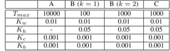
A B (k= 1) B (k= 2) C

Tmax 10000 100 1000 1000

Kw 0.01 0.01 0.01 0.01

Kh - 0.05 0.05 0.05

(6)

y

0 x

d

vector A

obstacle

Ax Ay

mobile object

Fig. 4. Simulation on obstacle avoidance

0 0.2 0.4 0.6 0.8 1

obatacle start place

learning data

Fig. 5. Learning data denoted by dots to avoid obstacle.

2) Obstacle avoidance and arriving at the designated place: As shown in Fig.10, the distanced1and the angleθ1

between mobile object and obstacle and the distanced2and

the angleθ2between mobile object and the designated place

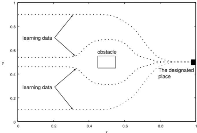
are selected as input variables. The problem is to construct fuzzy inference system that mobile object avoids obstacle and arrives at the designated place. From (operation) data, Fuzzy inference rules for each model are constructed from learning of data (200 points shown in Fig. 11). The number of partitions for each model is 5. As the same method as the above, the mobile object moves with the vector A at each step, whereAy ofAis output variable. The simulation

condition is shown in Table III.

Four tests after learning are performed as follows: (1)Test 1 is simulation for obstacle avoidance and ar-riving at the designated place when the mobile object stars from various places (See Fig.12). Fig.12 shows the results of moves of mobile object for starting places at (0.1,0),(0.2,0),· · ·,(0.8,0),(0.9,0) after learning. As shown in Fig.12, the test simulations are unsuccessful and successful for SIRMs and DIRMs models, respectively. (2)Test 2 is simulation for the case where the mobile object arrives at different designated place. Simulations arriving at the place (1, 0.35) different from the designated place (1, 0.5) in learning are performed for DIRMs model (See Fig.13). The results are successful as shown in Fig.13.

0 0.2 0.4 0.6 0.8 1

(a) SIRMs model

0 0.2 0.4 0.6 0.8 1

y

x (b) DIRMs model

Fig. 6. Simulation result for obstacle avoidance starting from various places learning

0 0.2 0.4 0.6 0.8 1

old place of obstacle new place

(a) SIRMs model

0 0.2 0.4 0.6 0.8 1

y

x (b) DIRMs model

(7)

0 0.2 0.4 0.6 0.8 1

y

x Goal point [0.3, 1.0]

Start point [0.9, 0]

Fig. 8. The obstacle moves with the vector (0.012, 0.02) at each step from starting point (0.9, 0) to arriving point (0.3, 1.0).

0 0.2 0.4 0.6 0.8 1

(a) SIRMs model

0 0.2 0.4 0.6 0.8 1

(b) DIRMs model

Fig. 9. Simulation for moving-obstacle avoidance.

(3)Test 3 is simulation for the case where the mobile object avoids obstacle placed at different place and arrives at the different designated place. Simulations with obstacle placed at the place (0.4, 0.4) and arriving at the designated place (1, 0.6) are performed for DIRMs model (See Fig.14). The results are successful as shown in Fig.14.

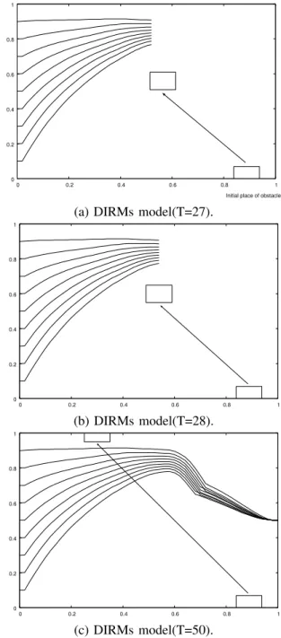
(4)Test 4 is simulation for the case where obstacle moves with the fixed speed. Simulations with obstacle moving as Fig. 8 and arriving at the place (1, 0.5) are performed. The results for the stepsT=27, 28 and 50 are shown in Fig.15. It means that simulations for obstacle avoidance are successful. Lastly, we performed the same simulations for the variable increase method for DIRMs model. As a result, all test sim-ulations are also successful in the variable increase method

y

0 x

d

vector A

obstacle

Ax Ay

mobile object

goal d2

2

1

Fig. 10. Simulation on obstacle avoidance and arriving at the goal.

0 0.2 0.4 0.6 0.8 1

y

x

learning data

obstacle

The designated place

Fig. 11. Learning data to avoid obstacle and arrive at the designated place (1, 0.35).

for DIRMs model. Therefore, the number 6 of modules for DIRMs model can be reduced to the model composed of 3 modules.

V. CONCLUSION

In this paper, a theoretical result and some numerical simulations including obstacle avoidance are presented in order to compare DIRMs model with SIRMs model. It is shown that there exists the difference of capability in the the-oretical means with EX-OR problem with two variables and in numerical simulation with two-category problems. Further, two types of obstacle avoidance problems are performed: The first problem is simply to avoid obstacle and the second one is to avoid obstacle and to arrive at the designated place. In the first problem, both SIRMs and DIRMs models are successful in all test simulations. In the second problem, there exists the difference of capability between DIRMs and SIRMs models in simulations. Further, DIRMs model with the variable increase method is also successful in all simulations. In the future works, the application to the other control problems and a proposal of the new generalized SIRMs model are considered.

REFERENCES

(8)

0 0.2 0.4 0.6 0.8 1

(a) SIRMs model

0 0.2 0.4 0.6 0.8 1

(b) DIRMs model

Fig. 12. Simulation for obstacle avoidance and arriving at the different designated place after learning.

0 0.1 0.2 0.3 0.4 0.5 0.6 0.7 0.8 0.9 1

0 0.2 0.4 0.6 0.8 1

Fig. 13. Simulation for obstacle avoidance with the different designated place (1, 0.35) from learning.

0.1 0.2 0.3 0.4 0.5 0.6 0.7 0.8 0.9 1

0 0.2 0.4 0.6 0.8 1

DIRMs.

0 0.2 0.4 0.6 0.8 1

0 0.2 0.4 0.6 0.8 1 Initial place of obstacle

(a) DIRMs model(T=27).

0 0.2 0.4 0.6 0.8 1

(b) DIRMs model(T=28).

0 0.2 0.4 0.6 0.8 1

(c) DIRMs model(T=50).

[2] C. Lin and C. Lee,Neural Fuzzy Systems, Prentice Hall, PTR, 1996. [3] M.M. Gupta, L. Jin and N. Homma, Static and Dynamic Neural

Networks, IEEE Press, 2003.

[4] J. Casillas, O. Cordon, F. Herrera and L. Magdalena,Accuracy Im-provements in Linguistic Fuzzy Modeling, Studies in Fuzziness and Soft Computing, Vol.129, Springer, 2003.

[5] B. Liu,Theory and Practice of Uncertain Programming, Studies in Fuzziness and Soft Computing, Vol.239, Springer, 2009.

[6] S. Araki, H. Nomura, I. Hayashi and N. Wakami, “A Fuzzy Model-ing with Iterative Generation Mechanism of Fuzzy Inference Rules,”

Journal of Japan Society for Fuzzy Theory and Systems, vol.4, no.4, pp.722–732, 1992.

[7] S. Fukumoto, H. Miyajima, K. Kishida and Y. Nagasawa, “A Destructive Learning Method of Fuzzy Inference Rules,”Proc. of IEEE on Fuzzy Systems, pp.687–694, 1995.

[8] K. Kishida, H. Miya jima, M. Maeda and S. Murashima, “A Self-tuning Method of Fuzzy Modeling using Vector Quantization,”Proceedings of FUZZ-IEEE’97, pp.397–402, 1997.

(9)

Connected Fuzzy Inference Model for Plural Input Fuzzy Control,”

Fuzzy Sets and Systems, 125, pp.79–92, 2002.

[11] N. Yubazaki, J. Yi and K. Hirota, “SIRMS (Single Input Rule Mod-ules) Connected Fuzzy Inference Model,”J. Advanced Computational Intelligence, 1, 1, pp.23–30, 1997.

[12] N. Shigei, H. Miyajima and S. Nagamine, “A Proposal of Fuzzy Inference Model Composed of Small-Number-of-Input Rule Modules”,

Proc. of Int. Symp. on Neural Networks: Advances in Neural Networks - Part II, pp.118–126, 2009.

[13] S. Miike, H. Miyajima, N. Shigei and K. Noo, “Fuzzy Reasoning Model with Deletion of Rules Consisting of Small-Number-of-Input Rule Modules,”Journal of Japan Society for Fuzzy Theory and Intelli-gent Informatics, pp.621–629, 2010 (in Japanese).

[14] H. Miyajima, N. Shigei, H. Miyajima, “An Application of Fuzzy Inference System Composed of Double-Input Rule Modules to Con-trol Problems,”Lecture Notes in Engineering and Computer Science: Proceedings of The International MultiConference of Engineers and Computer Scientists 2014, IMECS 2014, 12-14 March, 2014, Hong Kong, pp.23–28.