Delayed enhancement cardiac MRI: reduction of image artefacts in patients with irregular heart rate

(1)

UNIVERSIDADE DE LISBOA FACULDADE DE CIˆENCIAS

DEPARTAMENTO DE F´ISICA

Delayed Enhancement cardiac MRI: reduction of

image artefacts in patients with irregular heart rate

Andreia Calisto de Freitas

Dissertac¸˜ao

Mestrado Integrado em Engenharia Biomédica e Biof´ısica Perfil de Radiaç ões em Diagnóstico e Terapia

(2)

(3)

UNIVERSIDADE DE LISBOA FACULDADE DE CIˆENCIAS

DEPARTAMENTO DE F´ISICA

Delayed Enhancement cardiac MRI: reduction of

image artefacts in patients with irregular heart rate

Andreia Calisto de Freitas

Dissertac¸˜ao

Mestrado Integrado em Engenharia Biomédica e Biof´ısica Perfil de Radiaç ões em Diagnóstico e Terapia

Orientador externo: Professor Doutor Tobias Schaeffter, KCL Orientador interno: Professora Doutora Rita Nunes, IBEB, FCUL

(4)

(5)

Resumo

DE-MRI (do inglês delayed enhancement magnetic resonance imaging) consiste numa técnica de imagiologia de ressonância magnética (MRI do inglês Magnetic Resonance Imaging) com especial aplica¸cão em patologias card´ıacas.

Nos últimos anos, as técnicas de imagiologia de ressonância magnética tem desempen-hado um importante papel no diagnóstico e prognóstico médico. Caracter´ısticas vanta-josas tais como uma elevada resolu¸cão espacial, ausência de radia¸cão ionizante e múltiplas aplica¸cões impulsionaram o seu uso alargado a várias áreas da medicina moderna.

DE-MRI foi inicialmente desenvolvido para diagnóstico e avalia¸cão de enfarctes do miocárdio (vulgarmente denominado ataque de cora¸cão). No entanto, a aplica¸cao a doen¸cas isquémicas não é exclus´ıva, sendo que recentes estudos demonstraram a sua utilidade no diagnóstico de outras patologias card´ıacas tais como metástases card´ıacas, infeçcões virais e condi¸cões genéticas.

DE-MRI consiste geralmente na aquisi¸cão de imagens com pondera¸cão em T1 uti-lizando uma sequência IR (do inglês inversion recovery) após inje¸cão de um agente de contraste. Tal como o nome indica delayed enhancement distingue-se das técnicas ima-giológicas de contraste usuais uma vez que o momento de aquisi¸cão é atrasado por um determinado per´ıodo de tempo (geralmente entre 10 a 20 min) após inje¸cão do agente de contraste.

O agente de contraste mais frequente em DE-MRI é um composto à base de gadol´ıneo (Gd) chamado DTPA-Gd (do inglês diethylene-triamine-penta-acid gadolinium). O gadol´ıneo puro apresenta fortes caracter´ısticas paramagnéticas, magnetizando-se quando sob o efeito de um campo magnético exterior, sendo por isso natural a sua utiliza¸cão como agente de contraste em MRI. A utiliza¸cão de um agente de contraste permite obter

(6)

con-relaxa¸cão T1 dos protões circundantes. No entanto, é um composto altamente bio-tóxico e instável, sendo necessária a sua quela¸cão com o composto DTPA para o tornar seguro em aplica¸cões médicas.

Contudo, essa quela¸cão leva a que as moléculas de Gd apresente um elevado tamanho molecular, tendo por isso tendência a acumular em tecidos que sofreram enfarte (tecido necrótico) uma vez que estes possuem um alargado espa¸co extracelular em oposi¸cão ao miocárdio saudável.

Devido a esta distribui¸cão distinta do agente de contraste pelos tecidos card´ıacos é poss´ıvel obter o contraste de sinal entre o miocárdio que sofreu enfarcte e o saudável. Isto porque aquando o momento de aquisi¸cão, após o per´ıodo de atraso, o agente de contraste já terá sido eliminado dos tecidos saudáveis mas ainda permanece em elevadas concentra¸cões nos tecidos que sofreram enfarcte. Assim, a presen¸ca do Gd em maior concentra¸cão nestes tecidos irá reduzir o tempo de relaxa¸cão T1, reflectindo-se numa elevada intensitade de sinal em imagens com pondera¸cão T1.

Resumindo, numa imagem com pondera¸cão T1, o miocárdio que sofreu enfarcte irá apresentar elevada intensidade de sinal (tom claro na imagem) comparando com baixa intensidade de sinal (tom escuro na imagem) do miocárdio saudável.

De forma a auxiliar a distin¸cão de sinal entre os dois tecidos, uma sequência de gradientes IR é geralmente utilizada.

Uma sequência IR consiste na aplica¸cão de um impulso de radiofrequência de 180o despoletado por cada onda R na leitura electrocardiográfica (ECG) do paciente. Inicial-mente, a magnetiza¸cão longitudinal (Mz) possui um valor inicial denominado Mz0. Com

a aplica¸cão do impulso de inversão, o vector soma Mz é rodado em 180o _convertendo

Mz0 em −Mz0. Após o impulso de inversão, a magnetiza¸cão longitudinal irá então

recu-perar de −Mz0 a Mz0. O tempo de invers˜ao (TI) caracteriza o per´ıodo de tempo entre a

aplica¸cão do impulso de inversão e o momento de aquisi¸cão. O TI é selecionado de forma a coincidir com o ponto nulo de determinado tecido (usualmente o miocárdio saudável) permitindo anular o sinal desse mesmo tecido.

Resumindo, enquanto que por um lado a distribui¸cão diferenciada do agente de contraste permite aumentar a intensidade de sinal do miocárdio que sofreu enfarte, a aplica¸cão da sequência IR permite anular o sinal do miocárdio saudável. A jun¸cão de

(7)

ambos leva `a obten¸c˜ao do melhor contraste de sinal entre os dois tecidos.

Uma vez que DE-MRI desempenha um important papel na avalia¸cão de doen¸cas card´ıacas, a procura por uma melhoria na qualidade de imagem e ausência de artefactos, tem impulsionado vários projectos de investiga¸cão nos últimos anos. Algumas limita¸cões inerentes à técnica ainda permanecem por solucionar.

Tratando-se de uma t´ecnica cardiac triggered, irregulariedades no batimento card´ıaco influenciam directamente o comportamento da magnetiza¸c˜ao longitudinal e consequente sinal adquirido. Esta irregulariedade do sinal adquirido leva ao aparecimento de artefactos na imagem final quando reconstru´ıda.

Este projecto consistiu em avaliar de que forma irregulariedades no batimento card´ıaco influenciam o sinal adquirido e consequente aparecimento de artefactos na imagem final. Assim como posterior desenvolvimento e teste de um novo m´etodo de redu¸c˜ao de arte-factos das imagens em pacientes com um batimento card´ıaco irregular.

Diversos métodos de redu¸cão de artefactos através da otimiza¸cão do TI têm sido apresentados na comunidade cient´ıfica. Estes pretendem diminuir a dispersão do sinal do miocárdio saudável através de otimiza¸cão do TI para cada intervalo card´ıaco. No entanto, a otimiza¸cão do TI é dependente de T1 e a minimiza¸cão de varia¸cões do sinal do miocárdio saudável pode gerar artefactos devido ao sinal proveniente dos restantes tecidos que não foram corrigidos. O método de corre¸cão sugerido nesta disserta¸cão procura eliminar esse factor e otimizar dinamicamente o TI tendo em conta simultaneamente o sinal de vários tecidos.

O projecto consistiu primeiramente na constru¸cão de um ambiente de simula¸cão numérica e posterior implementa¸cão em scanner cl´ınico 3T utilizando fantomas exper-imentais.

O ambiente de simula¸cão encontra-se dividido em várias fun¸cões modulares. Uma primeira fun¸cão permite obter um registo simulado de ECG, representando o nosso pa-ciente virtual, podendo simular diferentes intervalos de tempo entre picos R com um determinado desvio-padrão (10%,20%...etc.) da média de batimento card´ıaco.

De seguida, uma segunda fun¸cão calcula a intensidade de sinal ao longo de cada janela de aquisi¸cão tendo em considera¸cão diversos parâmetros iniciais. Sendo os principais: TI, TR (tempo de repeti¸cão), TE (tempo de eco), o sinal de ECG e o factor de aquisi¸cão. O

(8)

factor de aquisi¸cão (N) permite definir o número de pontos do espa¸co-K adquiridos por cada janela de aquisi¸cão.

Uma terceira fun¸cão modular simula a aquisi¸cão de imagens 2D utilizando como input : um fantoma virtual, a intensidade de sinal previamente calculada e uma trajectória de aquisi¸cão no espa¸co-K. O fantoma virtual utilizado pretende representar um corte de curto eixo do ventr´ıculo esquerdo com três tecidos presentes: miocárdio que sofreu enfarte, massa de sangue no interior do ventr´ıculo e miocárdio saudável. De seguida, cada ponto de intensidade do sinal de cada vez pré-calculado através do T1 do tecido correspondente ´

e atribuido à máscara do tecido correspondente no fantoma virtual. Após soma das três máscaras de intensidade (três tecidos)e aplica¸cão de uma transformada de Fourier (FFT), o espa¸co-K final é obtido. Posteriormente, a trajectória de aquisi¸cão do espa¸co-K ´

e utilizada de forma a re-organizar a ordem em que este é preenchido. Por último, após transforma¸cão do espa¸co K através de uma transformada inversa de Fourier (IFFT) (do inglês Inverse Fast Fourier Transform), obtém-se a imagem final reconstruida.

A quarta fun¸cão modular aplica o método de corre¸cão de artefactos por otimiza¸cão do TI. O principal objectivo consiste em determinar o TI ótimo (T Iopt) que corresponde à

minimiza¸cão de varia¸cões do sinal (SSEtotal) dos vários tecidos considerados: SSEtotal=

W ∗ SSEmyocardium+ (1 − W ) ∗ SSEblood. Onde W ´e o factor que permite contra-balan¸car

a corre¸cão dando mais pondera¸cão a artefactos originários do sangue (W<0.5) ou do miocárdio saudável (W>0.5).

Por último, o método proposto foi implementado em scanner cl´ınico Philips 3T uti-lizando fantomas de gel de forma a representar os três tipos de tecidos (miocárdio que sofreu enfarte, sangue e miocárdio saudável). Para aquisi¸cão dos dados em scanner, os mesmos parâmetros de aquisi¸cão e sinal de ECG previamente calculados no ambiente de simula¸cão, foram utilizados.

Resultados obtidos com a simula¸cão numérica confirmaram que um batimento card´ıaco irregular afecta directamente o comportamento do sinal adquirido. Por exemplo para 50% de varia¸cão do batimento card´ıaco, o sinal do miocárdio saudável apresentou mais de 85% de dispersão em rela¸cão ao valor médio enquanto que o sangue revelou quase 30% de desvio. Verificou-se também que irregulariedades do batimento card´ıaco levam a maiores desvios de intensidade do sinal do miocárdio saudável e do sangue. Para além

(9)

disso, a simula¸c˜ao de imagens 2D revelou o aparecimento de artefactos com intensidade crescente de acordo com a intensidade de varia¸c˜ao do batimento card´ıaco.

Implementa¸cão do método de otimiza¸cão do TI foi executada com sucesso e revelou resultados positivos. Medi¸cões do n´ıvel geral de artefactos da imagem simulada para diferentes valores de W, permitiram concluir que o valor ótimo de W corresponde a 0,4. Para uma situa¸cão de 50% de varia¸cão do batimento card´ıaco e utilizando o método de corre¸cão com W=0,4, verificou-se uma diminui¸cão na varia¸cão do sinal do miocárdio saudável de 90 % para aproximadamente 25% e no sinal do sangue de 20% para menos de 10%. Tal como esperado, uma redu¸cão na varia¸cão de intensidade do sinal reflectiu-se na diminui¸cão da quantidade de artefactos na imagem final. Assim, verificou-se uma redu¸cão de 70% dos artefactos comparando com uma imagem não corrigida. Correspondendo 20 e 30 % mais comparando com corrigir apenas um tecido de cada vez, sangue e miocárdio saudável respectivamente.

Resultados similares foram obtidos nos dados experimentais adquiridos no scanner, com similar redu¸cão do n´ıvel de artefactos na imagem final. Medi¸cão do n´ıvel de artefactos nas imagens 2D dos fantomas experimentais levaram à conclusão que o método permitiu reduzir ainda mais o n´ıvel de artefactos comparando com os dados simulados. Com o método de otimiza¸cão do TI a W=0.4, a imagem apresentou uma redu¸cão de mais de 40% comparando com uma corre¸cão de apenas o miocárdio saudável.

Resumindo, os resultados experimentais foram coincidentes com os resultados simu-lados e parecem suportar a conclusão que a otimiza¸cão do TI tendo em conta múltiplos tecidos reduz com sucesso a quantidade de artefactos em imagens DE. No entanto, o es-tudo apresenta algumas limita¸cões. Os valores de T1 dos fantomas experimentais foram determinados através de uma sequência Look-Locker. No entanto, alguns resultados obti-dos sugeriram que a errada estima¸cão dos valores de T1 poderá ter ocorrido, o que levou ao desvio nos resultados obtidos.

Aspectos como variar a média do batimento card´ıaco para valores inferiores ou supe-riores, teste diferentes trajectórias de aquisi¸cão do espa¸co-K, novo teste dos valores de T1 dos fantomas, assim como determina¸cão dos parâmetros de aquisi¸cão para imagens in-vivo são importantes aspectos a considerar em estudos futuros.

(10)

alargado em termos da diminui¸cão de artefactos imagens DE-MRI. Concluiu-se que uma abordagem à otimiza¸cão de TI onde múltiplos tecidos são considerados apresenta vanta-gens relativamente à abordagem em que apenas a contribui¸cão do miocárdio saudável é tida em conta.

Palavras-chave: DE-MRI (Delayed enhancement Magnetic Resonance Imaging), Tempo de invers˜ao (TI), Enfarcte do mioc´ardio, Batimento card´ıaco irregular

(11)

Abstract

Delayed Enhancement Magnetic Resonance Imaging (DE-MRI) is a widely used imaging tool in the assessment of ischemic pathologies, crucial in distinguishing between infarcted and healthy myocardium [1]. Usually, T1 weighted images are acquired using an Elec-trocardiogram (ECG) triggered Inversion Recovery (IR) sequence after contrast agent injection which allows to increase signal contrast between the two tissues.

Since DE-MRI is cardiac triggered, heart rate (HR) irregularities directly affect signal behaviour. When HR varies, the time for the longitudinal magnetization (Mz) to recover is different for each cycle which leads to a different amount of magnetization available for acquisition. This irregular signal intensity can cause strong image artefacts.

Therefore, the purpose of this study was to develop a novel acquisition approach to compensate for HR variations using a multi-tissue model. Optimal Inversion Time (TI) values for each cycle were obtained by minimizing Mz variations of the healthy myocardium (SSEmyocardium) and blood (SSEblood): SSEtotal = W ∗ SSEmyocardium +

(1 − W ) ∗ SSEblood. The weighting (W) allows to correct more strongly for artefacts from

blood (W < 0.5) or myocardium (W>0.5) to achieve the best image quality possible. Simulations were performed to study signal behaviour and test the proposed multi-tissue correction approach. In addition, the method was also implemented on a 3T scanner and phantom experiments verified the simulated results.

The proposed multi-tissue method was successful when compensating for artefacts. For 30% HR variation scenario, it reduced image artefacts by approximately 70 % com-pared with a non-corrected image which is 20 and 45 % more than the single-tissue approach, only blood or healthy myocardium respectively.

(12)

presented approaches with a single tissue correction.

Keywords: DE-MRI, ischemic heart disease, inversion time (TI), irregular heart rate, arrhythmia

(13)

Acknowledgements

Although only one name appears at the front page, writing this dissertation would have been impossible without the crucial contribution from several people.

Firstly, many thanks to my supervisor Professor Rita Nunes for point out the way from the beginning, never forgetting some encouraging words when I was feeling lost.

I’m also extremely grateful to my external supervisor Professor Tobias Schaeffter, whose expertise carried this project to successful grounds and for the opportunity granted to work within such an amazing research group.

I would like to express my deepest gratitude to Dr. Christoph Kolbitsch for his patient, knowledge and perseverance even in the hardest hours of the project. From whom I learned that it is possible (or perhaps essential) to have passion for the work we do.

I would also like to thank to all the department staff for receiving me so nicely and making me feel part of the team. Many thanks to everyone in the cake club for their companionship and for making me leave King’s College London (KCL) not only with deep knowledge in medical imaging but also in baking!

I gratefully acknowledge financial support from the Eramus student interchange Grant. This dissertation is much more than one single project, it is the end of a journey that started almost 5 years ago. To all my colleagues (aka second family) at FCUL many thanks for all the fun moments. Thank you Catarina for the friendship and travelling along with me the same hard road. Thank you Carla for all the fun moments in London. Thank you Mariana for some (very!) important discussions about make up and croissants. Many thanks to my friends ”Mutantes” just for being there in the last few (ok...many, many) years.

(14)

(which is actually true!) but nevertheless was a major source of unconditional support. Finalmente mas nunca em último, esta tese é dedicada aos meus pais e irmã. Que sempre me ensinaram que o conhecimento não ocupa lugar.

Um grande obrigada a todos!

(15)

List of Figures

2.1 Representation of a healthy myocardium, acute and chronic myocardium infarction. . . 6 2.2 Example of DE-MR images with correspondent histological slices of MI

areas. . . 7 2.3 Acute and chronic transmural myocardium infarction shown with DE-MR

imaging. . . 8 2.4 Inversion recovery gradient echo sequence diagram. . . 11 2.5 Representation of T1 relaxation curves for healthy and infarcted myocardium. 12 2.6 Gadolinium concentration as a function of time after injection and

corre-spondent appropriate TI. . . 14 2.7 Schematic representation of longitudinal magnetization behaviour along a

repeated IR sequence. . . 15 2.8 Longitudinal magnetization behaviour when using R-R or 2R-R triggering. 16 2.9 Ghosting artefacts due to deficient breath holding and poor cardiac gating

in DE-MRI. . . 17 2.10 Multiple DE-MR images acquired correspondly to several different TI values. 18 2.11 Schematic representation of the longitudinal magnetization in a repeated

IR sequence considering a irregular heart rate. . . 19 2.12 Representation of longitudinal magnetization behaviour and correspondent

linear K-space sampling. . . 20 3.1 Numerical phantom representing short-axis view of the left ventricle. . . 25 3.2 Simulated 2D images with 30 % hear rate variation and a steady heart rate. 29

(18)

3.3 Simulated signal intensity curves along each acquisition window with a steady HR and a 30% HR variation with no correction method. . . 30 3.4 Signal intensity variation as a function of heart rate variation for the three

tissue types. . . 30 3.5 Simulated 2D images at 30% heart rate variation showing strong ghosting

artefacts. . . 31 3.6 Simulate signal intensity curves along each acquisition window considering

30% HR variation and correction method applied with W=0 and W=1. . 32 3.7 Artefacts intensity level for different W values considering each tissue

in-dividually and the sum of all tissues. . . 35 3.8 Signal deviatio as a function of different HR variation considering a

cor-rection method with only TI optimization or both parameters. . . 36 3.9 Signal intensity curves along each acquisition window applying correction

method with W=0.4. . . 36 3.10 Signal deviation over different heart rate variations considering correction

method with W=0.4. . . 37 3.11 Simulaed 2D images with 30% heart rate variation considering correction

method with W=0, W=1 and W=0.4. . . 38 4.1 Example of a 1D scan projection image. . . 40 4.2 Images of 1D scan projection acquired with a steady heart rate and 30%

heart rate variation. . . 42 4.3 Images of 1D scan projection acquired with a steady heart rate and 30%

heart rate variation. . . 42 4.4 Signal intensity curves from phantom experiments acquired with a steady

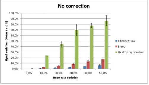
heart rate and 30% heart rate variation. . . 43 4.5 Measurements of signal variation (Y-axis) from phantoms experiments as

a function of hear rate variation (X-axis) without correction for the three tissue types. . . 44 4.6 Experimental phantoms 2D images acquired for a steady heart rate and

30% heart rate variation. . . 45

(19)

4.7 Signal intensity curves along each acquisition window acquired with 30% heart rate variation considering the correction method with W=0 and W=1. 46 4.8 Artefacts intensity level for different W values (phantom experiments)

mea-sured for each tissue individually and the sum of all tissues. . . 47 4.9 Signal intensity curves along each acquisition window acquired with 30%

HR variation and correction method with W=0.4. . . 47 4.10 Measurements of signal variation (Y-axis) from phantom experiments as a

function of heart rate variation (X-axis) with TI correction W=0.4 for the three tissue types. . . 48 4.11 Acquired phantom experiments 2D images for 30% heart rate variation

(20)

List of Tables

3.1 Acquisition parameters used for simulations. . . 26 3.2 Signal variation as a function of HR variation applying correction method

with W=0. . . 33 3.3 Signal variation as a function of HR variation applying correction method

with W=1. . . 33 4.1 Acquisition parameters used for phantom experiments acquisition. . . 40

(21)

List of Abbreviations

CAD Coronary artery disease.

DE-MRI Delayed Enhancement Magnetic Resonance Imaging. DTPA Diethylene-Triamine-Penta-acid.

ECG Electrocardiogram.

FCUL Faculty of Science, University of Lisbon.

Gd Gadolinium.

IBEB Institute of Biomedical Engineering and Biophysics. IR Inversion Recovery.

KCL King’s College London.

MI Myocardium infarction.

RF Radio Frequency.

SPECT Single photon emission tomography. SSE Sum of Squared Error.

TI Inversion Time.

(22)

(23)

Chapter 1 Introduction

The present dissertation describes the project developed by the author to complete an Integrated Master degree in Biomedical Engineering and Biophysics - Radiation in Di-agnosis and Therapy profile, at Faculdade de Ciˆencias, Universidade de Lisboa (FCUL), Portugal.

The project was developed at the Division of Imaging Sciences and Biomedical Engi-neering, KCL, United Kingdom (UK). This was under the LLP/Erasmus student inter-change program for a period of eight months between October 2012 and May 2013.

During this project a novel approach to reduce artefacts due to heart rate variations in DE-MRI was developed.

Professor Tobias Schaeffter, deputy head of the Division of Imaging Sciences and Biomedical Engineering, with extensive experience in imaging sciences was the external supervisor. Close collaboration with Dr. Christoph Kolbitsch, post-doctoral associate at the department, was also crucial for the project accomplishment.

Professor Rita Nunes, post-doctoral researcher at the Instituto de Biof´ısica e Engen-haria Biom´edica (IBEB), FCUL and assistant teacher at FCUL was the internal super-visor. Professor Nunes works mainly at IBEB but also has current projects at KCL, allowing to establish the contact between the two research groups.

(24)

CHAPTER 1. INTRODUCTION

1.1 Project background

Since the 1980s MRI has been used to assess myocardial infarction with the use of contrast agents [2]. Commonly, T1 weighted images are obtained using a cardiac triggered IR gradient echo sequence after contrast agent injection [3–5].

This leads to a high signal contrast and consequent distinction between the ocardium that has suffered irreversible infarction (necrotic tissue) and the healthy ocardium, being a useful tool for physicians to evaluate the extent of non-viable my-ocardium and therapeutic course in a wide set of cardiac pathologies.

Any cardiac MRI technique is challenging due to the cardiac and respiratory chest motion. This can be usually compensated for with cardiac triggering, where data is acquired in the period where the heart is more steady (mid-diastole), and breath hold or respiratory navigators [6].

However, patients with irregular heart rates still pose a major challenge for DE-MRI. Since it is cardiac triggered technique, irregular heart rate can directly influence the ac-quired MR signal. When the heat rate varies, the time for the longitudinal magnetization to recover is different for each cardiac cycle which leads to a different amount of magne-tization available at the time of data acquisition. This irregular magnemagne-tization behaviour leads to a variation of the acquired signal, causing strong artefacts when the final image is reconstructed [7].

As DE-MRI becomes a widely used cardiac imaging tool, the demand for high quality images increases proportionally and several studies have been presented to compensate for this limitation in the past few years [8–10].

Most methods compensate for this limitation by adapting the TI for each cardiac cycle to ensure the healthy myocardium signal is always nulled [8, 9]. Nevertheless this TI correction is T1 dependent and correcting for the healthy myocardium can create artefacts arising from other tissue types, such as from the blood pool.

The overall goal of the project was to develop a method to reduce artefacts due to arrhythmia considering a multi-tissue approach. The main goal is to correct the TI such that the magnetization available at acquisition remains as stable as possible. A more stable magnetization behaviour will translate in a final image with fewer and less

(25)

CHAPTER 1. INTRODUCTION

pronounced artefacts.

Firstly, a numerical simulation was built to study signal behaviour under the influence of irregular HR and develop the novel correction method. Secondly, the correction method was implemented at a 3T scanner using the same parameters. Experimental data from gel phantoms was used to validate simulated results.

1.2 Thesis outline

This thesis is divided into 5 chapters. Chapter 1 is the current chapter. A brief resume of the project background, respective supervisors and development is given.

Chapter 2 presents a background introduction to important concepts of DE-MRI. Technical aspects of the technique are explained such as medical applications, functioning of an IR sequence acquisition, choice of the TI and main limitations of DE-MR images. In addition, a brief explanation of current image artefacts correction methods is also given. Chapter 3 refers to the first portion of this dissertation study, the built of a numerical simulation environment. Methodology referring to the construction of the simulation environment as structure, main functions, mathematical description of the signal and parameters used, can be found in this chapter. In addition, the simulated results are also presented.

Chapter 4 presents the second portion of the study: phantom experiments in a 3T scanner. Both the methodology and results referring to the scanner experiments are shown.

Chapter 5 is a summary of this dissertation, including the conclusions drawn from the study, its contribution for the scientific community, main limitations and recommen-dations for future studies in the field.

(26)

Chapter 2 Delayed Enhancement MRI:

theoretical background

2.1 Introductory considerations

In DE-MRI, T1 weighted images are usually obtained using a cardiac triggered IR se-quence acquisition after contrast injection. DE imaging is most commonly used for dis-crimination between healthy myocardium and infarcted myocardium, for medical diag-nosis and therapeutic establishment purposes [1, 11].

As the name indicates, delayed enhancement imaging distinguishes itself from en-hancement imaging by delaying the acquisition by a certain period of time (usually be-tween 10 to 20 minutes) after contrast injection [12]. Therefore this technique allows to differentiate the tissues based on their distinct wash-out times [1]. A slower wash-out rate directly relates to a larger concentration of the contrast agent left in the tissue when acquisition is performed. Since the most commonly used contrast agents cause a short-ening effect of the T1 relaxation time, tissues with a higher concentration of the agent will present a shorter T1 value and thus a higher signal intensity in the final image.

In addition, a proper adjustment of the IR pulse sequence (i.e. selecting the inversion time such that the obtained signal from the healthy myocardium is null) increases the signal contrast between the healthy and infarcted myocardium.

The next sections of this chapter explore in depth these two main aspects of DE

(27)

CHAPTER 2. DELAYED ENHANCEMENT MRI: THEORETICAL BACKGROUND

imaging, as well as medical applications and limitations underlying this technique.

2.2 Ischemic heart disease and DE imaging medical

applications

Ischemic heart disease is the leading cause of death in adults in the world. In 2011 alone, approximately 7 million people died from ischemic heart disease [13].

Ischemic heart disease (or Myocardium infarction (MI)) is a heart pathology charac-terized by the malfunction of the heart wall due to partial or complete obstruction of the blood supply (ischemia). Ischemia causes a shortage of oxygen and vital nutrients to the correct functioning of the heart muscle.

In most patients, ischemic heart disease is related to another pathology called Coro-nary artery disease (CAD). CAD is characterized by the formation of an atherosclerosis plaque (substance made of cholesterol, fat and blood compounds) [14] which can lead to the hardening and narrowing of the coronary arteries [15]. The two coronary arteries (left and right) are responsible for irrigating the heart muscle. CAD and consequent malfunction of those arteries lead to heart muscle ischemia.

The myocardium can be affected to several degrees, from infarcted myocaridum (necrotic tissue) to hibernated myocardium. While hibernated myocardium presents minimum contractile function due to restricted blood supply but can recover after vas-cularization therapy, infarcted myocardium presents permanent cell destruction [16].

Additionally in clinical terms, distinction between acute and chronic MI is considered. Acute MI is usually characterized by necrotic cells (ruptured cellular membrane) and an enlarged extracellular volume. On the other hand, in chronic MI the absence of cells for a prolonged period led to the formation of a collagen matrix (fibrotic tissue) [1, 15]. Representation of both MI types and an healthy myocardium can be seen in Fig. 2.1.

Currently, Single photon emission tomography (SPECT) is one of the most common techniques used when assessing MI, since it can directly indicate metabolic function of the myocardium cells [17]. Nevertheless, it yields low spatial resolution images and does not provide high detailed information. MRI not only presents higher spatial resolution, it

(28)

Figure 2.1: Representation of a healthy myocardium with intact cells, acute MI with ruptured cell membranes leading to cellular death and chronic MI with formation of fibrotic tissue. (Image modified from [1])

also leads to higher reliability for some types of MI that are undetectable with SPECT. In a study by Wagner et al, MRI was reported to correctly identify 92% of sub-endocardial infarction segments while SPECT was only able to identify 30% [18].

Due to a higher spatial resolution, absence of ionizing radiation and multiplicity of applications, DE-MRI has become a well accepted alternative for cardiac diagnosis.

When dealing with MI patients, assessment of myocardium viability is crucial for predicting heart function recovery chance, deciding on a therapy course and calculating patient re-incidence rate. Assessment of myocardium viability consists in distinguishing between hibernated myocardium and infarcted myocardium.

In DE imaging, infarcted tissue usually presents enhancement after contrast injec-tion while hibernated myocardium does not. Previous studies proved that tissue showing enhancement (infarcted myocardium) continue to show lack of contraction even after vas-cularization therapy [19,20]. Thus supporting the theory ”bright is dead” where enhanced tissue is most likely irreversibly damaged [21]. In summary, enhancement in a certain portion of the heart wall in DE imaging is most likely related with infarcted myocardium. High reliability of MRI when matching infarct size to histology measurements (Fig. 2.2) was shown by Wagner et al. A high correlation coefficient (R=0.98) was reported between infarction size assessed with DE-MRI and assessed with histology measurements

(29)

[18].

Figure 2.2: (Top) Short axis view of the heart obtained with DE-MRI showing enhanced myocardium infarction. (Down) Correspondent histological slices with correspondent MI areas [18].

Another positive aspect of DE-MRI is that both acute and chronic MI show enhance-ment (Fig. 2.3). Nevertheless, some disagreeenhance-ment is still present regarding whether DE-MRI can be useful in distinguishing between the two of them. One current sugges-tion refers to using the presence of oedema (tissue swelling due to water accumulasugges-tion) as the differentiating factor since it is only present in acute MI. Since water usually presents a long T1 and T2 values comparing with healthy myocardium, signal contrast arises be-tween the oedema (acute MI) and the healthy myocardium. Current studies reported good results when identifying oedema in acute MI [22, 23]. This is accomplished by using a technique that uses both DE imaging and T2 weighted images.

DE-MRI can also be used to predict muscle function recovery after therapy. Previous studies presented evaluation of transmural extent of infarction area as a way to predict contractile improvement after therapy [24, 25]. For example, Choi et al. study concluded that when the percentage of tissue that showed improvement was reduced, the transmural enhanced infarction area increased. For segments with 1 to 20% infarction extent, around 67% showed contractible improvement but for 76% infarction extent in DE imaging, only 5% showed function improvement [24].

(30)

Figure 2.3: (a) Short axis DE-MRI view of the heart showing acute transmural MI. Enhance-ment of the infarcted myocardium is visible (arrows) compared to a null signal from the healthy myocardium (dark tone). (b) Short axis DE-MRI view of the hear from the same patient one year later (chronic MI). Infarcted myocardium continues to show enhancement and also shows thinning of the infarcted area compared to the acute MI phase [16].

DE might also be useful in patients with no previous history of myocardium infarction episodes but diagnosed CAD. It was reported that 81% of the patients with CAD, diag-nosed by X-ray angiography, showed delayed enhancement compared to only 8% in the control group. Therefore, DE might be a valid alternative to ionizing radiation methods when evaluating CAD patients and preventing future heart failure episodes [17].

While assessment of ischemic heart diseases is the most common usage for DE imaging, it is not exclusive and can be seen in a wide range of cardiac pathologies. A few examples are inflammatory diseases of the myocardium, cardiac neoplasms or genetic conditions [16].

2.3 Physiologic basis and contrast agent behaviour

Myocardium infarction assessment using DE imaging relies on different wash-out rates of the contrast agent and consequent effects on T1 values of the cardiac tissues.

The majority of contrast agents work by altering the T1 and T2 relaxation times of the surrounding tissues. According to the model described by Bloembergen, Purcell and

(31)

Pound [26], the effect of contrast agents on T1 and T2 relaxation times can be described by: 1 T 1 = 1 T1,0 + R1na (2.1) 1 T 2 = 1 T2,0 + R2na (2.2)

Where T1 and T2 are the relaxation times with contrast agent influence, T1,0 and T2,0

are the relaxation times in the absence of contrast agent, na is the agent’s concentration

and R1 and R2 are the agent’s relaxivity values. Relaxivity quantifies the ability of a

certain compound to change the relaxation rates of the surrounding proton spins per molar concentration.

The most commonly used agent in DE-MRI is a Gadolinium (Gd) based compound called DTPA-Gd. The gadolinium atom has seven unpaired electrons, giving it strong paramagnetic properties and becoming strongly magnetized when placed in an external magnetic field. Nevertheless, Gd is highly toxic in it’s pure state, being necessary to chelate it with another compound called Diethylene-Triamine-Penta-acid (DTPA). Thus making Gd thermodynamically more stable and biologically safer [27].

Gadolinium based agents comply to Equations 2.1 and 2.2 and present high values of relaxivity thereby shortening T1 and T2 times of surrounding tissues.

Distinct distribution of the agent in DE-MRI depends not only on the Gd kinetics but also on physiological characteristics of the heart tissues involved. Due to the chelation with DTPA, Gd presents a large molecular weight, having tendency to accumulate in tissues with larger extracellular volume [15]. Since tissues that suffered infarction usually present an enlarged extracellular space (Section 2.2), they tend to accumulate higher amounts of the contrast agent.

In addition, the delay period between contrast injection and acquisition ensures that most of the contrast agent has already washed out from the healthy tissue but remains in higher concentration in MI tissues.

In conclusion, tissues with higher Gd concentration (infarcted tissue) have a shorter T1 value and consequently appear bright on T1-weighted images. On the other hand,

(32)

tissues with longer T1 values (less Gd concentration) appear darker, such as the healthy myocardium. The blood pool tends to present an intermediate T1 value.

2.4 Inversion recovery pulse sequence and inversion

time

Distinct distribution of the contrast agent between the different heart tissues allows for the infarcted myocardium to be slightly more enhanced than the healthy tissue. In addition, an IR pulse sequence is usually used to achieve the best signal contrast possible between the two tissue types [28].

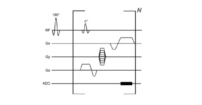
Inversion recovery is a gradient echo pulse sequence where a 180o pulse precedes a gradient echo read-out. However, 2D MR images relate to a large amount of data and image acquisition has to be divided into several sections (over several acquisition windows). In addition, the acquisition window length is limited by mid-diastole, thus a limit number of K-space lines can be sampled per cardiac cycle. Thereby the read-out portion is repeated N times to allow acquisition of multiple data points per inversion pulse (Fig. 2.4) [15].

Initially, the magnitude of the net vector of longitudinal magnetization is positive and described as M z0. Application of the inversion pulse flips the magnetization vector by

180o_{transforming M z}

0into −M z0. After the IR pulse, longitudinal relaxation occurs [15]:

Mz(t) = Mz,eq(1 − 2e−

t

T 1) (2.3)

Where T1 is the longitudinal relaxation parameter and Mz,eq the magnetization at

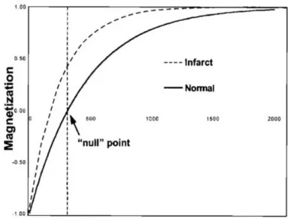
equilibrium. Longitudinal relaxation curves (Equation 2.3), without considering read-out, for healthy and infarcted myocardium can be seen in Fig. 2.5.

(33)

Figure 2.4: Inversion recovery gradient echo sequence diagram. Firstly an 180o _Radio

Fre-quency (RF) pulse is applied to cause inversion of the net Mz vector, followed by a gradient echo read-out (inside brackets). The brackets portion can be applied several times per cardiac cycle to allow the acquisition of multiple segments within the same inversion pulse. The ex-citation RF pulse is applied, flipping the available longitudinal magnetization towards the xy-plane by the angle defined by α. Secondly, the echo is obtained through application of a bipolar frequency-encoding gradient (Gx). Firstly to dephase the protons spins and the secondly as frequency read-out. Gy gradient defines the phase-encoding gradient that allows to define the K-space line that it is being sampled. The Gz gradient is the slice selection gradient allowing to select the 2D slice. Finally, the ADC (analogue to digital converter) allows for the signal to be acquired [15].

The time point where the magnetization is zero (null point) depends on T1 and can be used to null the signal from a chosen tissue. The time period between the inversion pulse and excitation is the TI. This is usually selected such that the healthy myocardium signal is null, relating to the best signal contrast between healthy and infarcted myocardium [1].

(34)

Figure 2.5: Longitudinal magnetization relaxation curves for healthy myocardium (longer T1) and infarcted myocardium (shorter T1) after application of an IR pulse. The ”null point” corresponds to the time point for which the healthy myocardium signal is null [2].

2.4.1 Selecting the time of inversion

Selecting the appropriate TI is a crucial step to obtain a good image quality and a diminished level of artefacts.

Nevertheless, several drawbacks can be encountered. Firstly, the TI varies from pa-tient to papa-tient and so it is empirically determined for each subject [29]. Secondly, it also depends on several factors such as: contrast agent administrated dose, cardiac function, time after contrast injection, among others [28].

Mathematically it is possible to determine the appropriate TI from its dependency of the T1 of the healthy myocardium. Following from Equation 2.3, the tissue signal is null when Mz(T Inull) = 0, therefore TI can be estimated:

Mz(T Inull) = Mz,eq(1 − 2e−

T Inull

T 1 ) = 0 (2.4)

T Inull = −T 1ln(2) (2.5)

However, in in-vivo situations, it is not possible to know the accurate value of T1 of the myocardium a priori.

(35)

Several methods are presented throughout the literature to determine the optimal TI, for example, using cine MR scout images or T1 mapping measurements [28, 30].

Using cine IR images to estimate TI is a trial and error technique. After the usual 180o

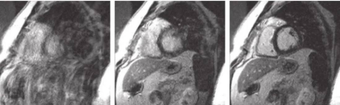
IR pulse is applied, a fast steady-state free precession readout is implemented allowing to acquire multiple images along the longitudinal recovery curve, correspondent to different TI values (Fig. 2.10). The optimal TI corresponds to the visually selected image where the healthy myocardium appears to have a null signal [28].

As an alternative, the TI can be estimated through direct T1 mapping measurements [15, 30] using a Look-Locker sequence [31]. This allows to more accurately estimate T1 of the healthy myocardium and correspondent adequate TI (Equation 2.5).

The incorrect selection of the inversion time can lead to image artefacts and mislead during evaluation of the myocardial infarction (Section 2.5).

2.4.2 Imaging time after contrast agent injection

As equally important as the selecting the correct TI, choosing the imaging time after contrast injection is another major concern in DE-MRI.

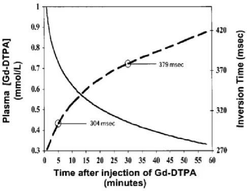
Each tissue signal intensity directly depends on the present Gd concentration level within the tissue at the time of acquisition (Section 2.3). However, Gd concentration doesn’t remain steady and gradually washes out with imaging time. Thereby, the chosen TI might no longer be adequate and needs to be adjusted if acquisition takes too long [2]. Figure 2.6 shows the direct relation between Gd concentration and the TI value. Exponential decrease of plasma Gd concentration with time (solid line) is based on real data acquired by Weinmann et al for a Gd injection dose of 0,125 mmol/Kg [32]. The dashed line describes the correct TI necessary to null the myocardium calculated from Gd concentration at a given time [33]. For example, at 5 minutes after injection, the correct TI is estimated to be approximately 304 ms.

The idea to keep in mind is that diminished Gd concentration translates to a weaker T1 shortening effect resulting in tissue with a longer T1 and consequent need to increase the TI [33]. Correct estimation of the TI might be possible but it is important to consider that it is transient for each cardiac cycle and if acquisition takes too long, it might no

(36)

longer be nulling the myocardium signal for the last data points acquired.

Figure 2.6: Concentration of Gd plasma as a function of time after injection (solid line) and appropriate TI for correspondent Gd concentration (dash line). As imaging time after injection increases, the adequate TI for a certain dose of Gd also increases [2].

In addition, another study suggested that imaging time after contrast injection can also affect infarct size estimation. Oshinki et al suggested that for a Gd dose of 0,03 mmol/kg, data should be acquired at 21 ± 4 minutes after injection so that the enhanced area matches true MI size. On the other hand, images acquired right after injection (within the 10 minutes range) overestimated infarcted size by 20-40 % [34].

In conclusion, both studies seem to suggest that imaging time after injection plays a crucial role in ensuring correct signal nulling of the myocardium.

2.4.3 Repeated IR time sequence and triggering

A repeated IR sequence is usually applied to allow acquisition of a segmented 2D image matrix over several acquisition cycles.

A schematic representation of a repeated IR acquisition is shown in Fig. 2.7.

Each IR pulse is triggered by an R-peak on the ECG signal. However, a delay period 14

(37)

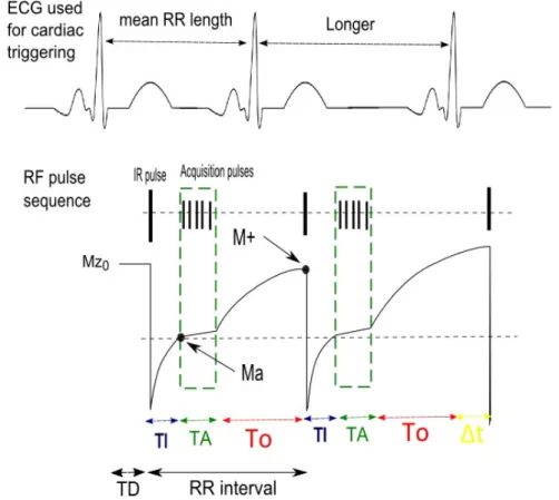
Figure 2.7: Schematic representation of longitudinal magnetization from the healthy my-ocardium along a repeated IR sequence. The first cycle represents a steady HR (mean R-R length) while the second cycle represents an irregular HR situation (longer interval than mean R-R).

(TD) introduced between the R-peak triggering and inversion pulse application, allows for acquisition to occur in mid-diastole. After the IR pulse, −M z0 is allowed to recover

until Ma (Mz available at acquisition) when the read-out sequence portion is applied. The TI is selected such that acquisition begins at the time point for which the healthy myocardium signal is null. The MR signal can then be acquired by flipping Ma towards the xy-plane (Mxy). During acquisition (dashed box), several consecutive acquisition pulses (α), equidistant by a time period TR, are applied to acquire multiple data points. Acquisition is set to last for a time period TA. Finally, the last Mxy point is allowed to recover until M+ (Mz available before the next inversion) for a period of time T0.

(38)

RR = T I + T A + T0 (2.6)

If the heart beat is irregular, an extra ∆t can either be positive (R-R interval is longer than mean R-R) or negative (R-R interval is shorter than the mean):

RR = T I + T A + T0 ± ∆t (2.7)

In terms of triggering, DE imaging can use R-R or 2R-R (Fig. 2.8). This means that the IR pulse can either be applied for every R peak occurrence (R-R) or for every other R peak (2 R-R). Using a R-R gating reduces the amount of time available between IR pulses which leading to incomplete magnetization recovery. On the contrary, a 2R-R gating allows for a more complete magnetization recovery and is specially recommended for tachycardia patients. However, 2 R-R gating does require twice the acquisition time [1].

Figure 2.8: (Top) Mz behaviour when R-R gating is used leading to incomplete magnetization recovery. (Bottom) Mz behaviour when 2R-R gating is considered, improving magnetization recovery and allowing to obtain higher signal intensity [1].

2.5 Image artefacts and limitations

A major concern in DE-MRI, as in any cardiac imaging modality, is the presence of image artefacts due to cardiac motion.

For DE-MRI restricting data acquisition to a so-called acquisition window placed dur-ing the mid-diastolic period is usually a successful compensation technique [6]. However,

(39)

not only there is cardiac motion but respiratory motion of the chest as well. The latter is usually compensated for by breath-holding or respiratory navigation approaches.

Nevertheless when those are deficient, specific artefacts can be identified. Deficient breath holding usually causes ghosting of chest area while poor cardiac gating causes ghosting of the heart itself (Fig. 2.9).

Figure 2.9: Image DE-MRI showing: (a) ghosting artefacts of the overall chest area due to deficient breath holding (b) ghosting artefacts of the heart itself due to poor cardiac gating (c) no ghosting artefacts due to acquisition with correct breath hold and gating [6].

When imaging tachycardia patients, it is crucial to use 2R-R or even 3R-R gating to allow for complete magnetization recovery. That will ensure higher signal intensity and less ghosting artefacts [1].

Patients with tachycardia also present another challenge to DE imaging since their mid-diastole period is usually shorter. To reduce ghosting due to heart movement, the acquisition window duration has to be shortened with less K-space lines sampled per window [6].

Another source of inaccurate images can be the incorrect choice of TI (Fig. 2.10). When the TI is selected too short (T I−3, T I−2 or T I−1), the healthy myocardium

presents a negative longitudinal magnetization value when the first α pulse is applied. Nevertheless, the measured SI corresponds to the magnetization magnitude, so in fact the healthy myocardium presents a higher signal intensity than the infarcted tissue. Thereby, as the TI becomes shorter, the signal of infarcted tissue will decrease until it reaches the null point. For an extremely short TI, the infarcted tissue appears null and the healthy myocardium enhanced (T I−3). On the other side, an excessively long TI (T I1, T I2 or

(40)

Figure 2.10: (Top) Signal intensity over time for three different tissue types: healthy my-ocardium, blood pool and infarcted tissue, considering multiple TI values. The signal magni-tude directly depends on the TI chosen. (Down) DE-MR images correspondent to the different TI values [28].

is not null. Both tissues will present a positive SI and consequently less image contrast. For the optimal TI (T I0) the infarcted myocardium shows enhancement (image

ar-rows) while the healthy myocardium presents a null signal [28].

However, even if all these limitations are compensated for, one major limitation re-mains. Since DE-MRI is cardiac triggered, irregular HR directly affects signal behaviour causing strong image artefacts.

In the theoretical situation where HR is completely steady, the interval between R-peaks is constant and so longitudinal magnetization has always the same time to recover. Therefore, the signal intensity (Ma) is the same for all cardiac cycles.

However if the R-R length varies, the amount of time for the longitudinal

(41)

tion to recover is different for each cycle (Fig. 2.11). If the R-peak occurs earlier than usual, the time available for Mz to recover is shorter than To. Therefore the Ma available at the next cycle will be higher. On the other hand, if the R-peak occurs later, Ma of the following cycle will have a lower intensity.

In summary, varying R-R lengths will lead to a variation of the acquired MR signal over several acquisition cycles.

Figure 2.11: Schematic representation of Mz behaviour over time in a repeated IR acquisition considering two different tissue types: healthy myocardium (black solid line) and infarcted myocardium (red solid line). For a patient with irregular heart rate, the cardiac cycles present different lengths thereby influencing Mz behaviour.

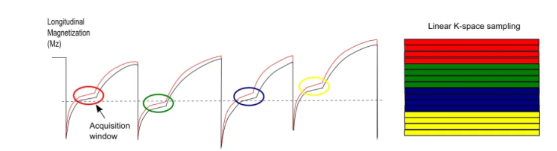
Thereby when sampling K-space, different segments will be assigned with different signal intensities (Ma) depending on their correspondent acquisition window (Fig. 2.12). As a result, sampling K-space with different signal intensities leads to strong artefacts when the final image is reconstructed.

To compensate for image artefacts due to HR irregularities is the main focus of this thesis.

(42)

Figure 2.12: Schematic representation of Mz behaviour over time using a repeated IR acqui-sition with irregular heart rate. In each cardiac cycle an acquiacqui-sition window (coloured circles) is considered where several data points are acquired. On the right side of the image a represen-tation of K-space linear sampling is shown. Different segments of K-space are filled with data from their correspondent acquisition window. Different colouring of the segments/acquisition windows represents different signal intensities.

2.5.1 Minimization of image artefacts due to irregular HR

A wide range of correction methods has been presented through the literature with posi-tive outcome in reducing image artefacts due to irregular HR and incorrect nulling of the myocardium.

A study by Krishnamurthy et al. reported positive results when applying a TI opti-mization method to reduce artefacts in arrhythmic patients [8]. The method consisted in dynamically adapting the TI for each acquisition cycle:

T Iopt = ln(2/(1 + exp(−RR/T 1))) ∗ T 1 (2.8)

Where R-R describes the length of the previous cardiac cycle and T1 the relaxation time of the tissue intended to be corrected. This formula was then used to accurately correct the myocardium signal. The study reported a decrease in artefacts intensity of 180 % with adaptive TI correction when compared without a correction method. My-ocardium/blood CNR also showed an improvement of approximately 70% with TI cor-rection.

Another recent study reported an alternative approach to dynamic TI optimization, where not only the TI is optimized for each cardiac cycle but also the inversion pulse angle (αIR) is considered [7]. The degree of αIR applied directly influences the amount

of Ma available and thereby the final signal intensity acquired. Thereby, optimization of 20

(43)

not only the TI but also the αIR can be useful to minimize signal irregularities.

TI optimization was be described by:

∆T Iopt = T 1ln

e−T 0T 1 − 2

e−T o−∆tT 1 − 2

!

(2.9) Inversion pulse angles optimization was described by:

cos∆αIR =

e−T 0T 1 − 1

e−T 0−∆tT 1 − 1

(2.10) With this optimization method, the study reported a reduction in the myocardium signal deviation from the mean value of 15 % to 2, 5% [7, 9].

However, both of these TI optimization methods are T1 dependent according to Equa-tions 2.8 and 2.9. Thereby, selection of the optimal TI that correctly nulls the healthy myocardium does not correspond to the optimal TI of the remaining tissues. Thus opti-mal correction of the healthy myocardium only reduces image artefacts arising from the healthy myocardium. Strong image artefacts may still arise due to signal variation of the non-corrected tissues.

Thereby, the proposed method in this thesis intends to compensate not only for a single tissue but multiple tissues simultaneously. By taking into account several tissues signals when optimizing the TI, artefacts arising from different tissue can be corrected and the overall artefacts level further reduced.

(44)

Chapter 3 IR DE-MRI simulation environment

3.1 Introduction and motivation

Due to DE-MRI wide range of medical applications and crucial role when assessing MI patients, demand on image quality and artefact compensation methods has increased.

Nevertheless, a major limitation remains when imaging irregular heart rate patients. If the heart rate is unsteady, signal intensity will be different for each acquisition cycle. In this case, different segments of K space are sampled with different signal intensities leading to strong artefacts when the final image is reconstructed (Section 2.5). The presence of such artefacts decreases image quality and misleads clinical diagnosis, thereby being of crucial importance to develop methods that aim to compensate for such artefacts.

Previous studies have presented compensation methods that dynamically adapt the TI in order to guarantee that the signal from healthy myocardium is always null. However, the choice of TI is T1 dependent and correcting for the healthy myocardium can still lead to artefacts arising from other tissues that were not corrected.

Therefore, this project intends to develop a novel artefacts reduction method that takes into account several tissue types. The main goal is to correct the TI for each cardiac cycle such that signal intensity remains as constant as possible. A multi-tissue approach is considered such that image artefacts arising from different tissue types can all be reduced simultaneously. In addition, the method also considers adapting two acquisition parameters (TI and α) to try to compensate for the maximum amount of artefacts possible.

(45)

CHAPTER 3. IR DE-MRI SIMULATION ENVIRONMENT

For the purpose of this study, a simulation environment was built by the author, modelling 2D DE-MRI acquisition using a cardiac triggered IR sequence.

The following sections of the this chapter present the methodology and results ob-tained with the construction of such simulation environment.

3.2 Methodology

The built simulation environment comprehended several levels of organisation in different functions such as: ECG triggering, mathematical description of a repeated IR sequence signal (Section 3.2.1) and 2D image acquisition (Section 3.2.2).

The first modular function, (ECG triggering), was responsible for generating a virtual ECG signal. Random time lengths between two consecutive R peaks were simulated with a standard deviation (10 to 50 %) around the mean heart rate [7]. Both the mean heart rate as well as the deviated distribution could be changed initially as input variables. Thus allowing to simulate multiple situations from a steady HR to a more irregular HR. This virtual ECG signal served as trigger to the following modular function (Section 3.2.1).

3.2.1 Mathematical description of a repeated IR signal

To allow for a quantitative prediction of the signal for different levels of HR irregularities, a second modular function (IR sequence signal ) modelled the MR signal behaviour for an IR sequence (Section 2.4.3).

SI was determined taking into account the longitudinal magnetization at excitation prior to data acquisition (Ma) as well as sequential calculation of transversal magnetiza-tion (Mxy) and recovering longitudinal magnetization (Mz) over the acquisition window

in consecutive cardiac cycles.

Longitudinal magnetization at excitation (Mz,n) of cycle (n) directly depends on the

longitudinal magnetization available before the IR pulse at the end of the previous cycle (n-1) (Mplus) [7] :

(46)

Mz,n= 1 + (Mpluscos(α) − 1)e

−T I

T 1 (3.2)

Where T0 corresponds to the mean R-R interval length, α is the excitation flip angle

and ∆t describes the difference between the varying R-R length and the mean R-R length (T0).

However during simulation implementation, the first cardiac cycle was set as an excep-tion since there is no previous cycle to recover from. Thereby, longitudinal magnetizaexcep-tion at acquisition (Mz,n) was set to [7]:

Mz,n = 1 + [(1 − e

−T o−∆t

T 1 )cos(180o)]e −T I

T 1 (3.3)

Nevertheless, equation 3.2 and equation 3.3 were only used to describe (Mz,n) for the

first data point acquired in each acquisition window.

The following points were calculated considering how the longitudinal magnetization (Mz,n) recovers from the previous acquisition pulse (α) [35]:

Mz,n= Mz,n−1e

−T R

T 1 cos(α) + M_z0(1 − e −T R

T 1 ) (3.4)

Regardless of the data point, each longitudinal magnetization (Mz,n) is brought to

the xy-plane and the transversal magnetization (Mxy) can then be calculated [35]:

Mxy = Mz,ne

T E

T 2∗sin(α) (3.5)

The number of repeated Mz,n and Mxy calculations (data points acquired) per

acqui-sition window was set by the variable N (Section 2.4).

Since acquisition lasts for a period of time (TA), it directly depends on the number of data points per window (N) and the time between consecutive excitations (TR):

T A = T R ∗ N (3.6)

Both the TR and N could be changed at the start of simulation as input variables.

(47)

3.2.2 Simulate 2D image acquisition

Signal behaviour at acquisition modelled earlier was then used to simulated 2D image acquisitions.

This third modular function (2D image acquisition) required as input the simulated ECG signal, the signal intensity previously calculated (Subsection 3.2.1), a numerical phantom and a K-space sampling trajectory.

A numerical phantom was implemented to mimic a short-axis view of the left ventricle representing three tissue types: fibrotic tissue, healthy myocardium and blood pool (Fig. 3.1).

Figure 3.1: Numerical phantom used in the simulation environment representing a short-axis view of the left ventricle with three different tissue types: fibrotic tissue (F), blood pool (B) and healthy myocardium (M).

The phantom was manually outlined from a scan image and a mask set to define the outlines of each tissue. Each mask was assigned with intensity of 1 and the remaining background set to zero. However for representation purposes, in Fig. 3.1 the tissue masks were assigned different intensities.

Secondly, each tissue mask was assigned with the signal intensity calculated (Section 3.2.1) for the correspondent T1 value of that tissue. This was done for each data point individually, followed by the sum of the three tissue specific signal masks. To the final image thus obtained, a 2D fast Fourier transform (FFT) was applied resulting in the

(48)

Parameters Value used

Mean heart rate 75 bpm

Matrix size 240 x 240 pixels

N factor 12 lines per window

Number of acquisition cycles 20

Fibrotic tissue (T1) 220 ms

Blood pool (T1) 310 ms

Healthy myocardium (T1) 550 ms

TE/TR 0/4.7 ms

Initial TI 270 ms

Initial excitation flip angle (α) 25 degrees

Start-up echoes 8

Upper boundary [40,450]

Lower boundary [0,150]

Table 3.1: Acquisition parameters used for simulations.

correspondent K-space matrix.

After this, the transformed K-space was modelled according to the chosen sampling trajectory, re-organizing data points by the order of acquisition set by the sampling trajectory. A simple linear cartesian trajectory was used in the simulation environment in similarity to the one used by the scanner. Finally, an inverse fast Fourier transform (IFFT) was applied to reconstruct the final image.

Parameter values used during simulation can be seen in Table 3.1. Upper and lower boundaries variables refer to a set of values defined during the TI optimization method; further description is available in Section 3.2.3. Since the T2* of the simulated tissues were unknown and for simplicity reasons, the TE was considered null. It was assumed that neglecting the T2 relaxation effect would not have a major effect on the final results, however it is a limitation of the simulation environment.

(49)

3.2.3 TI compensation method using a multi-tissue model

The method here suggested considers a multi-tissue approach of the dynamic TI opti-mization. The main purpose was to optimize TI such that signal intensity of several tissues remained as constant as possible.

This was achieved by minimizing the differences between the signal acquired with HR

variation (SItissue,%HRvariation) and the reference signal with no HR variation (SItissue,0%HRvariation).

This was accounted for using the Sum of Squared Error (SSE) for each tissue individually (SSEtissue):

SSEtissue = Σ(SItissue,%HRvariation− SItissue,0%HRvariation)2 (3.7)

Since a multi tissue approach was considered, the sum of squares total error (SSEtotal)

was calculated taking into account the (SSEtissue) not only for the healthy myocardium

but for multiple tissues.

All three tissue types could have been taken into account, nevertheless from signal behaviour results further discussed in Section 3.3.1, only the blood pool and healthy myocardium were considered for the correction:

SSEtotal = W ∗ SSEmyocardium+ (1 − W ) ∗ SSEblood (3.8)

Where W (weighting factor) allows to correct more strongly for artefacts arising from the healthy myocardium (W > 0.5) or from the blood pool (W < 0.5).

Thereby the main idea was to determine the optimal acquisition parameters (T Ioptand

α) that correspond to the minimization of the (SSEtotal) which minimises irregularities

in Ma.

A MATLAB integrated script called fminsearchbnd was used to calculate the opti-mized parameters. fminsearchbnd allows to search for the local minimum (X) around an initial value (X0) of an input function (fun) with a set of upper and lower boundaries (LB,UB):

(50)

In this study, this function was used for searching the value of TI (T Iopt) that

corre-sponds to the minimum of the function (SSEtotal):

[T Iopt, α] = f minsearchbnd(SSEtotal, parametersinitial, LB, U B) (3.10)

Where the array parametersinitial defined the initial parameters values around which

the function searches for a solution and [LB, U B] was the set of boundaries for the parameters search. Specific values used for these variables are shown in Table 3.1.

In addition to only optimizing the TI, another scenario was also tested where both acquisition parameters (TI and α) were optimized. Thus intending to study the effect of optimizing the flip angles as a way to further improve image quality. In the Table 3.1, UB and LB refer to the values used when optimizing both the TI and the excitation flip angle (α) simultaneously, where [0,40] boundaries refer to α and [150, 450] to TI. In the case where the optimization of the TI was considered, UB and LB only included the values [150] and [450].

3.2.4 Evaluation of signal deviation and image artefacts

The effect of irregular heart rate in signal behaviour was quantified by calculation of the signal standard deviation. The standard deviation allowed to quantify how much the signal deviates (σ) from the mean (µ) signal [36]:

σ = v u u t 1 N N X i=1 (xi− µ)2 (3.11)

To obtain signal deviation percentage wise, σ was divided by µ and multiplied by 100. Secondly, a method was devised to quantify image artefacts intensity (Fig. 3.2). A reference image (simulated with steady HR) was subtracted to each simulated image with HR variation. Thus obtaining an image that solely holds the artefacts intensity (Fig.3.2 (c)). The overall artefacts intensity was quantified by calculating the mean value of this final image.

This quantification method of artefacts level was used to compare the our TI opti-mization method with non-corrected images.

(51)

Figure 3.2: (a) Simulated 2D image of the left ventricle considering a steady heart rate. (b) Image simulated for 30% HR variation. Gray scale was adapted to visually enhance image artefacts. (c) Image solely holding the artefacts intensity obtained subtracting image (a) from image (b).

3.3 Results and discussion

3.3.1 Influence of irregular HR on signal behaviour and image

quality

Simulation of a repeated IR signal acquisition according with the experimental method-ology described in section 3.2.1 was successfully accomplished. Signal intensity curves were simulated with steady heart rate (reference signal) and with heart rate variation.

Reference signal along each acquisition window acquired with no heart rate variation can be seen in Fig. 3.3 (a,b,c). As expected for a regular HR, all signal curves within each tissue type showed the same intensity (signal curves overlap) meaning Ma remained constant for all cycles.

For 30 % heart rate variation and no method of correction, signal curves showed different intensities and no longer overlap (Fig. 3.3 (d,e,f)). This means that Ma was irregular and the acquired signal presents different intensities.

In order to quantify the effect of irregular HR in signal behaviour, signal variation was measured (Section 3.2.4) for all three tissue types considering different HR variation values (Fig. 3.4).

Results shown that both HR variation and signal variation present a direct relation, where a higher HR variation leads to a higher signal deviation, specially for the my-ocardium (ex: 50 % HR relates to almost 90% signal deviation).

Delayed enhancement cardiac MRI: reduction of image artefacts in patients with irregular heart rate

Delayed Enhancement cardiac MRI: reduction of

image artefacts in patients with irregular heart rate

Andreia Calisto de Freitas

Delayed Enhancement cardiac MRI: reduction of

image artefacts in patients with irregular heart rate

Andreia Calisto de Freitas

Resumo

Abstract

Acknowledgements

Contents

List of Figures

List of Tables

List of Abbreviations

Chapter 1

Introduction

1.1

Project background

1.2

Thesis outline

Chapter 2

Delayed Enhancement MRI:

theoretical background

2.1

Introductory considerations

2.2

Ischemic heart disease and DE imaging medical

applications

2.3

Physiologic basis and contrast agent behaviour

2.4

Inversion recovery pulse sequence and inversion

time

2.4.1

Selecting the time of inversion

2.4.2

Imaging time after contrast agent injection

2.4.3

Repeated IR time sequence and triggering

2.5

Image artefacts and limitations

2.5.1

Minimization of image artefacts due to irregular HR

Chapter 3

IR DE-MRI simulation environment

3.1

Introduction and motivation

3.2

Methodology

3.2.1

Mathematical description of a repeated IR signal

3.2.2

Simulate 2D image acquisition

3.2.3

TI compensation method using a multi-tissue model

3.2.4

Evaluation of signal deviation and image artefacts

3.3

Results and discussion

3.3.1

Influence of irregular HR on signal behaviour and image

quality