Automatic Sleep Apnea Detection and Sleep Classification using the ECG and the SpO2 Signals

(1)

1

Universidade Nova de Lisboa

Faculdade de Ciências e Tecnologia

Departamento de Engenharia Electrotécnica

Automatic Sleep Apnea Detection and Sleep

Classification using the ECG and the SpO2 Signals

Dissertation for a Masters Degree in

Computer and Electronic Engineering

Lara Andrea da Silva Simons

Supervisor: Prof. Doutor Arnaldo Batista

(2)

(3)

3

Supervisor: Prof. Doutor Arnaldo Batista

Departamento de Engenharia Electrotécnica

da Faculdade de Ciências de Tecnologia

(4)

4

You may not have thought about it, but people sure sleep a lot. Imagine...if on the average, people sleep 8 hours a day, they are sleeping away 1/3 of their life. How much is that? Well, 8 hours of sleep every day is the same as 233,600 hours of sleep by the time you are 80 years old. That's the same as sleeping 26.67 years!!! We also dream about 4-5 times a night: that is the

same as 116,800 to 146,000 dreams by the time you are 80 years old!!!

(5)

5

Agradecimentos

Ao Professor Arnaldo Batista, na qualidade de orientador científico, agradeço a

oportunidade concedida para a realização deste trabalho, a dedicação e o

profissionalismo demonstrado, assim como a amizade e motivação, sem deixar de

salientar a enorme disponibilidade apresentada para resolução dos problemas inerentes a

realização da tese, principalmente nos momentos de maiores dúvidas, sem duvida o meu

grande mentor neste último período do curso.

Aos meus colegas de curso, pela colaboração, amizade e solidariedade tão

importantes na difícil vida académica, que certamente irá deixar muita saudade.

À Prof.. Cristina Barbara e à sua equipa pelo apoio incondicional que me deram,

sem elas este trabalho não teria sido possivel.

Ao Carlos Mendes pelo grande suporte incondicional que me ofereceu na

realização da tese.

Por fim quero agradecer de forma especial, à minha mãe Maria de Lurdes da

Silva Simons, ao meu pai Jorge Arnaldo Simons, a minha irmã Sarah Andrea da Silva

Simons e ao meu namorado Nuno Vieitas pelo apoio e amor incondicional que sempre

(6)

6

Acknowledgments

To Professor Arnaldo Baptista, as scientific advisor, I would like to thank the

opportunity granted to carry out this work, his dedication and professionalism shown, as

well as friendship and motivation. I also have to point out the availability he has always

shown in helping resolving any problem or doubt concerning this thesis, especially

when the major questions arose. He has definitely been my greatest mentor during this

last part of my degree.

To my colleagues for their cooperation, friendship and solidarity in such a

difficult stage of academic life, that will certainly be missed.

To Dr. Cristina Barbara and her team for the unconditional support – without

them this work would have not been possible.

To Carlos Mendes for the great unconditional support you gave me on

completion of the thesis.

And finally, in a special way, to my mother Maria de Lurdes da Silva Simons, to

my father Jorge Arnaldo Simons, to my sister Sarah Andrea da Silva Simons and my

boyfriend Nuno Vieitas for their unconditional love and support – they were vital to

(7)

7

Figures Index

Figure 2.1.1 ... 24

Figure 2.3.1 ... 25

Figure 2.3.2 ... 26

Figure 3.1.1 ... 28

Figure 3.1.2 ... 29

Figure 4.1.1 ... 31

Figure 4.2.1 ... 32

Figure 4.2.2 ... 33

Figure 4.2.3 ... 33

Figure 4.2.4 ... 34

Figure 4.2.5 ... 35

Figure 4.2.6 ... 35

Figure 4.2.7 ... 36

Figure 4.2.8 ... 36

Figure 4.2.9 ... 37

Figure 4.2.10... 37

Figure 4.2.11... 38

Figure 4.2.12... 38

Figure 4.2.13... 39

Figure 4.2.14... 39

Figure 4.2.15... 40

Figure 4.2.16... 41

Figure 4.2.17... 42

Figure 4.3.1 ... 42

Figure 4.3.2 ... 43

Figure 4.3.3 ... 44

Figure 4.3.4 ... 44

Figure 4.3.5 ... 45

Figure 4.3.6 ... 45

Figure 4.3.7 ... 46

Figure 4.3.8 ... 47

(10)

10

Figure 4.3.10... 50

Figure 4.3.11... 51

Figure 4.3.12... 51

Figure 4.4.1 ... 53

Figure 4.4.2 ... 54

Figure 4.4.3 ... 56

Figure 4.4.4 ... 57

Figure 4.4.5 ... 58

Figure 4.4.6 ... 59

Figure 4.5.1 ... 60

Figure 4.5.2 ... 61

Figure 4.5.3 ... 61

Figure 4.5.4 ... 62

Figure 5.1 ... 67

Figure 5.2 ... 68

Figure 5.3 ... 69

Figure 5.4 ... 69

Figure 5.5 ... 70

Figure 5.6 ... 71

Figure 5.7 ... 71

Figure 5.8 ... 72

Figure 5.9 ... 72

Figure 7.1 ... 73

Figure 7.2 ... 74

Figure 7.3 ... 75

Figure 7.4 ... 76

Figure 7.5 ... 76

Figure 7.6 ... 77

Figure 7.7 ... 78

Figure 7.8 ... 79

Figure 7.9 ... 80

Figure 7.10 ... 81

Figure 7.11 ... 82

(11)

11

Figure 7.13 ... 84

Figure 7.14 ... 85

Figure 7.15 ... 85

Figure 7.16 ... 86

Figure 7.17 ... 87

Figure 7.18 ... 87

Figure 7.19 ... 88

Figure 7.20 ... 89

Figure 7.21 ... 90

Figure 7.22 ... 91

Figure 7.23 ... 92

Figure 7.24 ... 93

Figure 7.25 ... 93

Figure 7.26 ... 94

Figure 7.27 ... 95

Figure 7.28 ... 95

Figure 7.29 ... 96

(12)

(13)

13

Tables Index

Table 1.3.1 ... 18

Table 2.1.1 ... 24

Table 2.1.2 ... 23

Table 4.3.1 ... 52

(14)

(15)

15

ABSTRACT

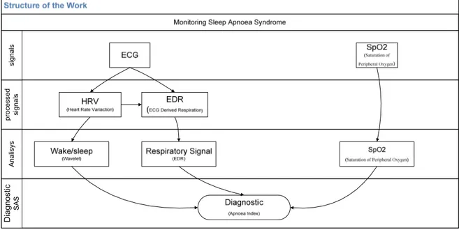
The present work describes the aspects to implement a system that can be used

as a swift and accessible screening tool in patients whose complaints are compatible

with OSAS (Obstructive Sleep Apnea Syndrome). This system only uses two signals,

electrocardiogram (ECG) and the saturation of oxygen in arterial blood flow (SPO2).

This system would be applied for the ambulatory automatic screening of OSAS, which

currently are done in a Hospital environment, with a substantial waiting list. The system

also would overcome the time consuming visual sleep scoring that contributes for the

mentioned waiting list. We have developed a system that automatically detects OSAS

based on the ECG and SpO2. However this system has to be paired up with another that

detects the awake/sleep/REM periods (also based on the ECG), which is also part of this

work. This last component has proved to produce results that are complex to classify,

for which there is still a lack of research work. However we have described the

necessary algorithms, and have used state-of-the-art signal processing tools, such as

(16)

(17)

17

1 Introduction

1.1 Introduction of the theme and Justifications

Obstructive sleep apnea syndrome (OSAS) is a clinical condition deemed by

international statistics to affect 4% of middle-aged men and 2% of middle-aged women 1,2,3

. OSAS is presently a serious public health concern, one which is under-diagnosed.

It is believed that around 93% of women and 82% of men suffering from OSAS are

undiagnosed 4. The definitive diagnosis is established in patients with a suggestive

clinical report and confirmed by polysomnography (PSG), demonstrating the apneas

associated with the physiological disorders. However, PSG is performed in a Sleep

Laboratory, being very expensive, and demanding considerable human and technical

recourses, not being readily available 2,3. Therefore, it is necessary to find other

diagnose methods for OSAS, which are simpler and available sooner to patients – and

that is the goal of this work. The purpose is to develop a system that can help diagnose

OSAS with very few signals (two: ECG and SPO2), that are easily obtained; a system

where the patients do not have to leave their homes and that is less expensive.

1.2 Specified Questions

 Which signals to use?

 How can we diagnose OSAS with the less signals possible?

 Which tools will we use to withdraw as much information as possible from

the two signals used?

 Can we obtain a Hypnogram from the ECG signal?

 Can we obtain a signal corresponding to the respiration signal from the

complex QRS (complex QRS is a structure on the ECG that corresponds to

(18)

18 proce sse d s ignal s Diagnostic SAS Anal isy s s igna ls

1.3 The Purposes of the Research

1.3.1 Main Purpose

The purpose of this work is to be able to diagnose OSAS, in a simple and

inexpensive way. The system developed must be able to diagnose OSAS with only two

signals (ECG e SPO2).

1.3.2 Specific Purposes

The specific purposes are:

a) To eliminate the noise of the ECG;

b) To use the wavelet’s tool, producing the Hyponogram from the ECG

signal;

c) To use the ECG-derived respiration (EDR) technique to detect apnea and

hypopnea

d) To determine the indexes of oxygen saturation in the arterial blood

stream.

Table 1.3.1 sums up the purposes of the work developed and every technique used

herein.

(19)

19

1.4 Organization of the Thesis

The outline of this thesis is as follows.

Chapter 1 provides a general overview of the present work, preliminary aspects,

relevance of the theme and its structure. Chapter 2 gives a brief description of sleep

definitions and their structure, as well as the apnea classification, and oxygen

desaturation. The typical representation of the ECG signal is also discussed. Chapter 3

briefly describes the theory concepts of wavelet analysis and EDR. Chapter 4

introduces the algorithm design, explaining all functions that compose this algorithm,

while in Chapter 5 the flowchart of each function representing that algorithm is

presented. Chapter 6 contains a small manual for software user interface. Chapter 7

provides the results of our modeling. The conclusions and guidelines for future work are

presented in Chapter 8.

(20)

(21)

21

2 Basic Medicine Notions

2.1 Sleep and its Structure

2.1.1 Sleep

Sleep is a natural state of bodily rest observed throughout the animal kingdom. It is

common to all mammals and birds, and it is also seen in many reptiles, amphibians and

fish, birds, ants and fruit-flies. Regular sleep is essential for survival. 5 However, its

purposes are only partly clear and are subject of intense research.6

2.1.2 Stages of Sleep

In mammals and birds the measurement of eye movement during sleep is used to

divide sleep into the two broad types of Rapid Eye Movement (REM) and Non-Rapid

Eye Movement (NREM) sleep. Each type has a distinct set of associated physiological,

neuronal and psychological features.

Sleep proceeds in cycles of REM and the four stages of NREM, the order normally

being:

Stages 1 -> 2 -> 3 -> 4 -> 3 -> 2 -> REM

In humans, this cycle lasts, on the average, 90 to 110 minutes7, with a greater

amount of stages, where stage 4 presents itself early in the night and more REM stages

later in the night. Each phase may have a distinct physiological function.

Allan Reachtschaffen and Anthony Kales originally outlined the criteria for

indentifying the stages of sleep in 1968. The American Academy of Sleep Medicine

(AASM) updated the staging rules in 2007.

The criteria for REM sleep include not only rapid eye movements but also a rapid

low voltage EEG. In mammals, at least, low muscle tone is also a sign. Most memorable

dreaming occurs in this NREM stage, which accounts for 75-80% of the total sleep time

in normal human adults. There is relatively little dreaming during the NREM sleep

stage. NREM encompasses four stages; stages 1 and 2 are considered ‘light sleep’ and 3

(22)

22

an EEG, unlike REM sleep which is characterized by rapid eye movements and relative

absence of muscle tone. In NREM sleep there are often limb movements, and

parasomnias, such as sleepwalking, may occur.

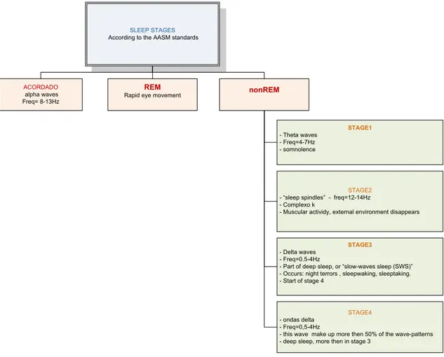
NREM consists of four stages, according to the 2007 AASM standards:

SLEEP STAGES According to the AASM standards

ACORDADO

alpha waves Freq= 8-13Hz

REM

Rapid eye movement

nonREM

STAGE1 - Theta waves

- Freq=4-7Hz - somnolence

STAGE2

- “sleep spindles” - freq=12-14Hz - Complexo k

- Muscular actividy, external environment disappears

STAGE3 - Delta waves

- Freq=0.5-4Hz

- Part of deep sleep, or “slow-waves sleep (SWS)” - Occurs: night terrors , sleepwaking, sleeptaking. - Start of stage 4

STAGE4

- ondas delta - Freq=0,5-4Hz

- this wave make up more then 50% of the wave-patterns - deep sleep, more then in stage 3

Table 2.1.1 – NREM and its four stages, according to the 2007 AASM standards

The method used to detect these stages is the Polysomnography, or PSG. This is a

multi-parametric test applied to the study of sleep; the test result is called a

polysomnogram. The PSG monitors many body functions including brain activity

(EEG), eye movements (EOG), muscle activity or skeletal muscle activation (EMG),

heart rhythm (ECG), and the breathing function or respiratory effort during sleep.

Here are some examples of different sleep states: awake, asleep, complex k, and

(23)

23

Table 2.1.2 – Examples of different sleep states: awake, asleep, complex k, and spindles.

Passing stage awake to

stage asleep

Spindles (rapid wave),

sleeping stage 2

Complex k, stage 2

(24)

24

2.1.3 Sleep Structure and Hypnogram

A Hypnogram is a diagram that summarizes the stages of sleep recorded in the

sleep laboratory. It is a graphic representation of the sequence of the various stages of

sleep (non-REM and REM). Figure 2.1.3 shows an example of a Hypnogram.

Figure 2.1.1 – Hypnogram.

2.2 Respiratory Rules

These rules are obtained by the American Academy of Sleep Medicine, Manual

for the Scoring of Sleep and Associated Events.

2.2.1 Scoring apneas

To score apneas, the event duration is measured from the nadir preceding the

first breath, which is clearly reduced, to the beginning of the first breath that

approximates the baseline breathing amplitude.

To score an apnea, there has to be a drop in the peak thermal sensor excursion by

>= 80%, the event has to last at least 10 seconds, and at least 90% of the event’s

duration have to meet the amplitude reduction criteria for apnea. There are 3 types of

apneas:

 Obstructive Apnea – if it meets the apnea criteria and it is associated with

continued or increased inspiratory throughout the entire period of absent

airflow.

 Central Apnea – if it meets the apnea criteria and it is associated with

absent inspiratory effort throughout the entire period of absent airflow.

 Mixed Apnea – if it meets the apnea criteria and it is associated with

absent inspiratory effort in the initial portion of the event, followed by

(25)

25

2.2.2 Oxygen Desaturation

To detect a desaturation there has to be a >=4% desaturation from pre-event

baseline.

2.3 The ECG Signal

In order to use this signal it is important to be aware of the typical representation

of the ECG signal, so that it is possible to understand all techniques and further

techniques that can be applied to an ECG signal.

2.3.1 Typical Representation of the ECG

In figure 2.3.1 it’s possible to understand the representation of a typical ECG

signal.

Figure 2.3.1 – A typical representation of an ECG signal.

All these waves are very important for the studies undergone in this present work.

2.3.2 The QRS Complex

The QRS complex is a structure on the ECG that corresponds to the

(26)

26

the atria, the QRS complex is larger than the P wave. A normal QRS complex has a

duration of 0.08 to 0.12 sec (80 to 120 ms). Figure 2.3.2 represents the QRS complex.

(27)

27

3 Theoretical Concepts

3.1 The wavelets

A wavelet is a mathematical function used to divide a given function or

continuous time signal into different frequency components and to study each

component with a resolution that matches its scale. A wave transform is the

representation of a function by wavelets. The wavelets are scaled and translated copies

of a finite-length or fast-decaying oscillating waveform. Wavelet transforms have

advantages over traditional Fourier transforms for representing functions that have

discontinuities and sharp peaks, and for accurately deconstructing and reconstructing

finite, non periodic and non-stationary signals.

The Fundamental idea behind wavelets is to analyze to scale. The wavelet

analysis procedure is to adopt a wavelet prototype function, called an analyzing wavelet

or mother wavelet. Temporal analysis is performed with a contracted, high-frequency

version of the prototype wavelet, while frequency analysis is performed with a dilated,

low-frequency version of the same wavelet. Because the original signal or function can

be represented in terms of a wavelet expansion (using coefficients in a linear

combination of the wavelet function), data operation can be performed using just the

corresponding wavelet coefficients. And if one further choose the best wavelets adapter

to the data, the coefficient below a threshold, the data is sparsely represented. This

sparse coding makes wavelets an excellent tool in the field of data compression.

3.1.1 Wavelet versus Fourier Transform

The fast Fourier transform (FFT) and the discrete wavelet transform (DWT) are

both linear operations that generate a data structure that contains log2n segments of

various lengths, usually filling and transforming it into a different data vector of length

2n.

The mathematical properties of the matrices involved in the transforms are

similar as well. The inverse transform matrix for both the FFT and the DWT is the

(28)

28

function space to a different domain. For the FFT, this new domain contains basis

functions that are sines and cosines. For the wavelet transform, this new domain

contains more complicated basis functions called wavelets, mother wavelets, or

analyzing wavelets.

There is another similarity between both transforms. The basis functions are

localized in frequency, making mathematical tools such as power spectra (how much

power is contained in a frequency interval) and scalograms (to be defined later) useful at

picking out frequencies and calculating power distributions.8

The most interesting dissimilarity between these two kinds of transforms is that

individual wavelet functions are localized in space. Fourier sine and cosine functions

are not.

One way to see the time-frequency resolution differences between the Fourier

transform and the wavelet transform is to look at the basis function coverage of the

time-frequency plane.9 Figure 3.1 shows a windowed Fourier transform, where the

window is simply a square wave. The square wave window truncates the sine or cosine

function to fit a window of a particular width. Because a single window is used for all

frequencies in the WFT, the resolution of the analysis is the same at all locations in the

time-frequency plane.

Figure 3.1.1 -Fourier basis functions, time-frequency tiles, and coverage of the time-frequency plane.

An advantage of wavelet transforms is that the windows vary. In order to isolate

signal discontinuities, one would like to have some very short basis functions. At the

same time, in order to obtain detailed frequency analysis, one would like to have some

very long basis functions. A way to achieve this is to have short high-frequency basis

(29)

29

transforms. Figure 3.1.2 shows the coverage in the time-frequency plane with one

wavelet function.

Figure 3.1.2- Wavelet basis functions, time-frequency tiles, and coverage of the time-frequency plane.

One thing to remember is that wavelet transforms do not have a single set of basic

functions like the Fourier transform, which utilizes just the sine and cosine functions.

Instead, wavelet transforms have an infinite set of possible basis functions. Thus

wavelet analysis provides immediate access to information that can be obscured by

other time-frequency methods such as Fourier analysis.

3.2 The EDR method

Knowledge of respiratory patterns would be clinically useful in many situations

in which the ECG, but not respiration, is routinely monitored. We describe a

signal-processing technique which derives respiratory waveforms from ordinary ECGs,

permitting reliable detection of respiratory efforts. Central and mixed apnea, hypopnea,

and tachypnea may be identified with confidence. In many cases, obstructive apnea and

changes in tidal volume are also clearly visible in the ECG-derived respiratory signal

(EDR).

This algorithm extracts approximate respiration signal from a single-lead ECG

using measurements across a fixed window. The window defines the QRS complex and

by default extends from -40ms to +40ms (relative to each R-wave). If the sample rate of

the ECG data is low (e.g. 100Hz) then one may wish to use the T-wave as the basis for

the EDR signal (since this part of the ECG is more slowly-changing than the QRS

(30)

(31)

31

4 Functions

Description

and

Interpretation

4.1 Function Architecture

The present work was organized, as shown in figure 4.1, where the titles stand for the

Matlab function names.

Eliminacao_ruido Outputs: Vector_zeros template hrv ecg_sem_ruido artefacto hdr_final hdr_final_sem_ruido RR_interp Output: RRI_interp spo2_sem_ruido_ecg Output: Spo2_sem_ruido simson_lara_sem_thorax Output: Sinalresp_final wave_cwt_lara Outputs: C_VLF C_LF C_HF C_LF_HF hipnograma Output: Hipo amplitude Outputs: resp_M resp_m amplitude_y indice_apeneia saturacao_spo2 Output: Indice_saturacao

Figure 4.1.1- Work Organization.

There is a main function that eliminates all noise from the ECG signal, and

constructs an ECG signal without artifact beats. When the ECG is noise free, there are

three main purposes to be achieved by this work:

1. To produce a respiration signal using EDR technique, and detect if there is any

apnea;

(32)

32

3. And to compute the Oxygen Desaturation Indices (ODI).

4.2 Eliminating the EGC noise

Our data is obtained from patients that underwent an all night recording session.

In this context, continuous data is acquired. This data is prone to be contaminated with

the artifacts that arise from sources such as unmanageable patient movements and

electrode displacement. This is one of the hardest tasks in this kind of work. There is

very little information on how to clear a signal from all types of noise, and many sorts

of noise can be found in a signal. Therefore, it is of the utmost importance to eliminate

the artifact contaminated beats from the signal in order to initiate all the further

computing that is required, without the noise that would bring several errors to the

aforementioned processing.

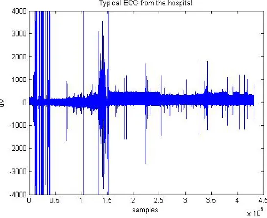
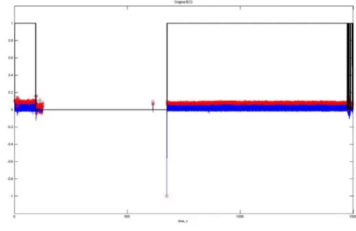
Figure 4.2.1 represents a typical ECG signal from a patient for a night session. It

is possible to observe various types of noise that need to be eliminated, in order to carry

out all the further processing.

(33)

33

The ECG signal is a cardiac cycle coordinated by a series of electrical impulses

produced by specialized heart cells found within the sino-atrial and the atrioventricular

nodes. Therefore, the ECG signal is a cycle of heart beats, as observed in figure 4.2.2

and figure 4.2.3.

Figure 4.2.2- Schematic representation of a Normal ECG

Figure 4.2.3- Patient ECG signal

The elimination of the ECG noise starts by eliminating the various parts of the

signal that differ from the typical representation of the ECG, so the first computing

performed is to detect all R picks in the signal. To detect those R picks an existing

function qrsdetect was applied. The results can be found in figure 4.2.4. This

(34)

34

open source code repository. Under test the function revealed to be stable and accurate

enough for our purposes.

As observed, this function works the best when the signal has no noise, since

noise causes the function to detect several types of wrong peaks, detrimental to the

results of the computing process.

Figure4.2.4- Detection of R peaks

One of the purposes of this function is to make a distinction between the good

and the bad peaks detected. After getting the vector that contains all peaks, there has to

be a way to identify and eliminate the bad ones, so that the signal can be freed from this

interference.

The algorithm that identifies and eliminates this type of noise works as follows:

1. Get a vector with all the R peaks invoking an existing function qrsdetect,

(figure 4.2.5 top)

2. Get a vector with the difference between R peaks, that is, get the Heart

Rate Variability (HRV);

3. Distinguish the good HRV from the bad one, which can be done since the

(35)

35

4. The purpose is achieved when the signal is split into pieces, which

should represent one cardiac cycle (figure 4.2.2). Figure 4.2.5 bottom

represents a split signal. The vector that contains the split signal is a

vector herein called beat (figure 4.2.5 bottom )

Figure 4.2.5- The ECG signal with artifact beats. Graphic 1 – ECG signal (blue), R-peaks (red) and vector that is zero when the artifacts occur (black); Graphic 2 – The splited ECG signal

Figure 4.2.6- Correlation Algorithm. Graphic 1: the obtained template; Graphic 2: All the separated beats, including the noisy ones; Graphic 3: Good beats only; Graphic 4: Bad beats only

5. Once, the signal is all split, by getting the mean of the vector beat, it is

obtained the template that will serve to compare with the entire beat

(36)

36

6. Correlation has the biggest computational load. This takes a long time

processing. Therefore, it is very difficult to process an entire night sleep

with standard pc’s. The result can be seen in figure 4.2.6.

7. After getting a vector with only good beats, all the good ones are

connected and the signal is freed from the artifact beats (figure 4.2.6 –

graphic 3 good beats, graphic 4 bad beats)

However, another type of noise can occur, as seen in figure 4.2.7. It happens when the

electrode comes off, for some reason, during a night sleep, making the signal flat in the

respective interval.

Figure 4.2.7- Another type of Noise – zeros

(37)

37

Figure 4.2.9- Original ECG with Noise

This is another type of noise that has to be eliminated. Figure 4.2.8 (bottom)

shows how the algorithm results: the flat zone was eliminated and the bears put

together.

Figure 4.2.9 represents an original ECG signal with some noise and zeros, the

red dots represent the R waves location.

Figure 4.2.10 zooms in on figure 4.2.9, where R peaks, representing noise

(yellow rectangle) can be seen.

(38)

38

Figure 4.2.11 also zooms in on figure 4.2.9 – One can see some noise in this part

of the signal; zeros represent noise as well (yellow rectangle).

Figure 4.2.11- Zoom of figure 4.2.9, yellow rectangle represents different types of noise.

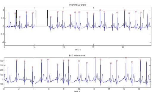
Finally, it is possible to see the algorithm at work in figure 4.2.12. When the

rectangular signal (black signal) is 1, it represents a good signal; when it is 0 (zero) it

represents noise.

(39)

39

Eventually, an ECG signal with reduced noise level is obtained; ready to be used

in further processing, as seen in Figure 4.2.13.

Figure 4.2.13- Result after elimination of the ECG noise.

It is important to mention that the noise was removed from the ECG signal, and

the parts with no noise placed together. This decision was taken because the intervals

needed for further processing are the R-R ones. Therefore, the difference between the

peaks will be the object of further computing. Initially, zeros were placed where

artifacts was detected, figure 4.2.14.

Figure 4.2.14- ECG with no noise.

(40)

40

But this decision was quickly reversed, because the R-R intervals would be

affected. This is why the good parts of the ECG signal were attached. This function

would work better if, instead of using the template obtained from ALL beats, it used the

template with only the good beats. This creates a problem for the computing process,

because in order to obtain a template with only the good beats the function would have

to be processed twice. It would have to get a template with the mean of all the beats, by

correlation, get a vector only with the good beats and get a new template with the mean

of the good beats and finally, by correlation once more, remove the artifacts beats of the

ECG signal. Figure 4.2.15 shows what happens when an ECG has too much noise.

(41)

41

In figure 4.2.15 (graphic 4) it can be seen what can happen if the ECG is

contaminated with severe noise, the template that is obtained by the mean of all beats, it

not the best.

Graphic 1 – ECG signal (blue) and selection function (black);

Graphic 2- ECG Signal where the artifact beats where eliminated and removed;

Graphic 3- Represents the HRV signal;

Graphic 4-The template obtained;

Graphic 5-The vector containing all the beats;

Graphic 6-The vector with the good beats:

Graphic 7-The vector with the bad beats only.

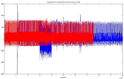
The ECG signal without noise then becomes out of phase with the original ECG,

and with less samples. This will most likely bring about problems in the future when

comparing these results with the hospital results, since the noisy epochs in the visual

scoring done by the Hospital Cardiopneumologists are replaced by the previous ones,

thus maintaining the signal length, which is not the case of our algorithm. Figure 4.2.16

shows the difference between the original data set and the one after removing the noisy

heart beats. . Figure 4.2.17 is zoomed version.

Figure 4.2.16- portraits the original ECG signal (blue), and the ECG signal after applying the

(42)

42

Figure 4.2.17- Zoom over Figure 4.10 (ylim([-600 600]))

4.3 Calculation of the Respiration Signal

It was our desire, in an early stage, to get the respiration signal by using

wavelets. But the signals obtained at the hospital were filtered in the band where the

respiration signal is present. We have demonstrated, after some testing, this result. Even

though this tool could not be used with these signals, another one could, the EDR. The

EDR used in this project has already been explained in chapter 3.2.

4.3.1 The EDR

To use this technique (EDR - Copyright Ben Raymond, March 2000 This file is

free software);several elements are required: R-R intervals, an ECG signal free from

different types of noise (achieved by previous function described in chapter 4.2), the

QRS onset and offset, and the ECG frequency. Figure 4.3.1 represents the onset and

offset waves in an ECG beat reference.

(43)

43

A standard function can be used to detect the onset and offset of the QRS:

sinalresp_final_1=edr(hdr_final',ecg_sem_ruido,[-40 40],fa);

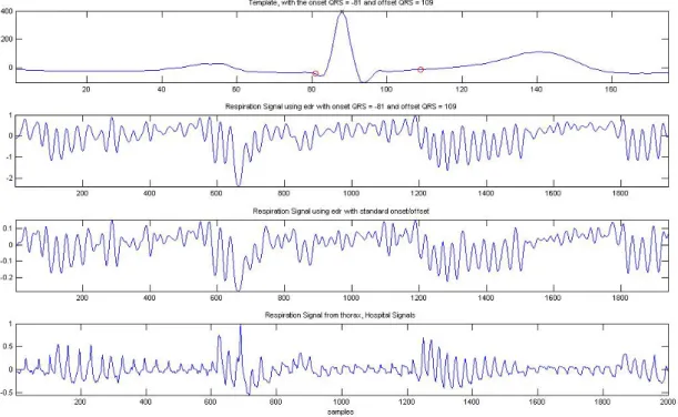
Figure 4.13 shows the respiration signal obtained from the EDR with the onset,

offset of the QRS standard, and the respiration signal from the thorax (signal obtained

by plethysmography sensor) of a patient. When observing figure 4.3.2 one has to take

into account the fact that the respiration signal obtained by the EDR is out of phase with

the thorax signal, due to the missed ECG beats, eliminated due noise. There is a good

accordance between the plots.

Figure 4.3.2- The EDR versus the Thorax signal.

To improve these results, the onset and offset must not be standard, but linear.

The onset and the offset must be calculated according to each template. To make that

calculation, an algorithm developed by Carlos Mendes (a colleague of mine studying

high resolution ECG in the same department) was used. This algorithm consists of (see

(44)

44

Figure 4.3.3- The normal ECG’s timing and shape.

1. Detects R peak;

2. Detects the maximum slope between point 1 and point 2;

3. Detects S peak;

4. From S peak, when the slope is smaller than it is the offset - in this case point 3;

5. To find the onset, the same algorithm is used, but symmetrically,

between R peak and Q peak.

The results, as seen, for one beat, in figure 4.3.4, are much better when using

this algorithm. The apnea is already visible in graphic 2, and one must keep in mind that

graphic 2 is out of phase with graphic 4.

Figure 4.3.4- The EDR with standard and non standard onset and offset. Graphic 1 – Template (blue) and the onset and offset detected in (red); Graphic 2 – EDR signal with a non standard onset and offset;

Graphic 3 – EDR signal with a standard onset and offset; Graphic 4 – Thorax signal

(45)

45

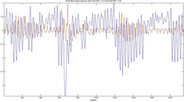
Figure 4.3.5- Red: Plethysmography respiration signal. Blue: EDR signal with linear onset/offset

detection.

Figure 4.3.5 shows in red the Plethysmography respiration signal, and in blue the

EDR signal with linear onset/offset detection. Despite not being clear in Figure 4.3.4,

this EDR version produces a respiration signal that better follows the original signal.

Since the EDR signal represents one sample for each heart beat this

un-homogeneous sample rate is much lower than the plethysmography signal (100Hz).We

have therefore to interpolate the signal to the same sampling rate of the

plethysmography signal to be able to compare both. Figure 3.3.6 shows on the top the

interpolated signal and on the bottom the original signal.

(46)

46

.Figure 4.3.7 shows the interpolated signal red along with the original Plethysmography

signal. We can see that the respiratory signal that the interpolated signal detects all the

respiratory cycles.

Figure 4.3.7-EDR Interpolated (red) and Plethysmography (blue).

Finally, we proceed to develop a function to detect apnea.

4.3.2 Number of Apnea

The purpose of this function is to detect the type of apnea. As it was described in

chapter 2.2.1, to score an apnea there has to be a drop in the peak thermal sensor

excursion by >= 90% and the event has to last at least 10 seconds. To achieve this goal,

the known function was used:

res = nbmaxima(t,f,position)

This function was developed by Jeremie Bigot, from the University Paul Sabatier, in

France. There are three principles in this function:

1. A point is maximum in a strict sense if the points that are immediately on

its left and right sides are smaller than it.

(47)

47

Xj is maximum in a strict sense if x(j-1)<xj and x(j+1)<xj

2. A point is a left maximum if it is bigger than the point on its left side and

equal to the point on his right side.

Example: Xj is left maximum if x(j-1)<xj and x(j+1)=xj

3. A point is a right maximum if it is bigger than the point on its right side

and equal to the point on its left side.

Example: Xj is left maximum if x(j-1)=xj and x(j+1)<xj

The function was developed to calculate the respiration amplitudes. Figure 4.3.8,

graphic 1 represents the respiration’s signal with its maximum and minimum detected,

and graphic 2 represents the correspondent respiration amplitudes.

These respiration amplitudes will be used to detect apnea events.

Figure 4.3.8- The Respiration Signal and the correspondent respiration amplitudes.

(48)

48

When the amplitude vector is obtained, it is possible to detect apnea events. The

algorithm used to detect the apnea consists of:

1. Initially, the amplitude vector contains all amplitudes;

2. Using the “find” function (Matlab function) it returns all the indices

whose amplitude is lower than 90% when compared to the baseline. It is

rather difficult to define a baseline; normally it is done manually, by an

expert. In this case, the baseline is obtained by calculating the average of

the first ten samples. This can cause some problems, if the scoring starts

with an apnea event;

3. Finally, by applying the “diff” function (Matlab function) to the vector

and dividing it by the sample frequency, a vector is obtained, containing

all the times the amplitude is lower than 90% when compared to the

baseline. All those bigger than 10 seconds correspond to an apnea event.

Figure 4.3.9 shows the algorithm running. The output variable ‘indice_apeneia’

is zero. No apnea events can be seen. In graphic 1 the EDR interpolated signal is

showed with the maxima (red) and minima (green) of the respiratory signals, graphic

represents the respiratory cycles, graphic 3 shows the apnea index.

Figure 4.2.10 represents the same situation with a signal with two apnea events

the output variable ‘indice_apeneia’ is two. As described before, an apnea event is

(49)

49

Figure 4.3.9- The Respiration Signal with no apnea events (see text).

(50)

50

Figure 4.3.10- The Respiration Signal with two apnea events (see text).

Lastly, using a plethysmography signal (Hospital Signal) as an input signal for

the function developed to calculate the respiration amplitudes, it is possible to observe

that the algorithm works correctly. Figure 4.3.11 represents the thorax signal and figure

4.3.12 represents a zoom out from figure 4.3.12, being possible so observe the

respiration signal and its constitution.

(51)

51

F

Figure 4.3.11- The thorax Signal. The yellow rectangle is zoomed in the figure 4.3.12.

(52)

52

For the above patient, it is possible to check in table 4.3.1 that the results are

rather satisfactory and acceptable.

Output from matlab

Polysomnography Report (hospital)

Table 4.3.1 - Comparison of the results.

4.4 Calculating the Hypnogram

In recent studies11 the electrocardiogram (ECG) has been used to classify sleep

into different states: Wake, REM and Sleep. These studies are recent and information

concerning autonomic changes is scarce when trying to classify sleep stages.

After extensive research, the purpose of this part of the work is to study the ECG

and be able to classify the three sleep stages (Wake, REM and Sleep). This autonomic

function was based on time-frequency analysis of the RR-Interval series, using the

power components in very-low-frequency range (0,005-0.04Hz), low-frequency

(0.04-0.15 Hz), and high-frequency ((0.04-0.15-0.5 Hz).

4.4.1 The RR-Interval Series

The R waves were automatically detected at the ECG, chapter 4.2, and their

occurrences as a function of time composed the RR interval series (RRI). RRI was

interpolated by equally spaced samples, and its time-frequency decomposition was

performed by a continuous wavelet algorithm. The power was calculated in 3 standard

(53)

53

1. VLF - very-low-frequency range (0.005-0.04Hz),

2. LF - low-frequency (0.04-0.15 Hz),

3. HF - high-frequency (0.15-0.5 Hz).

In figure 4.4.1, it is possible to observe the RRI Interpolated (graphic 1) and the

continuous wavelet used db5 (graphic 2). This is a reference plot only, and the wavelet

scalogram reveals no particular information, since it refers to an all night RRI and all

the frequency bands. The RRI was interpolated to 4 Hz and the interest band limited to

0.5 Hz.

Figure 4.4.1- RRI Interpolated (graphic 1) and the continuous wavelet (graphic 2), for an all night session.

The frequency bands were extracted from the EEG signal via continuous wavelet

transform with DB5. Figure 4.4.2, graphic 1 represents the RRI interpolated and graphic

2, 3 and 4 represent the power in the 3 standard frequency bands. For further studies, if

necessary, the blue signal in graphic 2, 3 and 4 is the wavelet power, the red signal is

the wavelet power using a 30 second sliding window, and in each window the average

is calculated. And finally, the green signal is the power frequency using a window every

(54)

54

Figure 4.4.2- Graphic 1 – RRI interpolated, Graphic 2 – wavelet power frequency band (0.005-0.04) blue signal power frequency band, red signal using a sliding window of 30 seconds and green signal using a window of 30 seconds with no overlap. Graphic - 3 power frequency band (0.05-0.15) blue signal power

frequency band, red signal using a sliding window of 30 seconds and green signal using a window of 30 seconds with no overlap. Graphic - 4 power frequency band (0.16-0.5) blue signal power frequency band, red signal using a sliding window of 30 seconds and green signal using a window of 30 seconds

(55)

55

Subsequently, it is possible to analyze the frequency bands to create rules for the

elaboration of the Hypnogram

4.4.2 The Hypnogram

The final goal of this chapter is to create a Hypnogram using the three frequency

bands (VLF, LF, HF) and the LF/HF ratio described in chapter 4.4.1. There are no

standard values for these parameters values in the wake, sleep and REM stages. The

purpose of this chapter is to make a contribution in this area, still in need of extensive

research. After studying various papers and documentation 11, it was verified that the

parasympathetic nervous system activity increases progressively and the sympathetic

nervous system activity decreases after falling asleep. In order to obtain a Hypnogram a

set of rules has to be created according to the alteration in frequency bands during

changes in wake, sleep and REM stages. It is known, that the high frequency band is

close to the respiration frequency, and represents the parasympathetic activity. The low

frequency includes information of the parasympathetic and sympathetic activity. The

sympathetic balance is defined by the quotient of the low frequency and the high

frequency. Lastly, very high frequency is defined as the mental and physical activity.

At first, after studying several papers on this subject, it was necessary to visually

observe the wavelet frequency bands and the respective curves of the VLF, LF, HF and

the LF/HF. It is possible to observe in figure 4.4.3 what happens to frequency bands in

(56)

56

Figure 4.4.3- Manual Monitoring: graphic 1- VLF, graphic 2 - LF, graphic 3 – HL and graphic 4 – LF/HF

Initially, when the visual scoring was done, there were 4 states: awake, REM,

light sleep and deep sleep. But since the three main states for sleep apnea are the awake,

REM and sleep ones, those were the ones defined. Rules had to be created to distinguish

between each state.

1. During the awaken state, the mental and physical activity is very high; this

corresponds to the VLF band; the parasympathetic activity (HF band) and the

LF band are very low. VLF is high and HF and LF are very low.

2. During the REM state, the mental and physical activity is high (lower then while

awake), and the sympathetic balance is high. VLF is high (but lower then

awake) and LF/HF is high.

3. During the sleep state, mental and physical activities (VLF band) are low, and so

is the sympathetic balance (LF\HF band). The parasympathetic activity (HF

band) is high. VLF is low, LF\HF is low and HF is high.

acordado

REM

light light

(57)

57

The energy in each band and for each epoch was devided in four steps: Very

High, Low and Very Low. This scoring was applied to each of the frequency

bands.

All these states were computed so that it is possible to generate an automatic

hypnogram using the ECG signal. A major problem arose; how can the Hypnogram

signals be compared? Initially (chapter 4.2) were the algorithm detected noise in the

ECG signal, those parts were deleted from the ECG signal and the ‘good’ parts were

placed together, so there is missing data. On the other hand, the Hospital hypnograms

do not have missing data, since all the artifact epochs were replaced by previous ones. If

a hypnogram is obtained from the ECG signal, the two graphics cannot be compared if

artifact data has been removed. Figure 4.4.4 shows the reference Hypnogram and our

version. The results are obviously not good for reasons we proceed to explain.

Figure 4.4.4- The two Hypnograms; graphic 1 - hypnogram signal of a patient under study, graphic 2 – hypnogram obtained from the ECG signal

In chapter 4.2 the artifact beats were eliminated and removed. There is a vector,

stored in the memory, containing all information of the eliminated beats. That vector

(58)

58

with a 200Hz sampling frequency. But our Hypnogram has a 4 Hz sampling frequency

so it is necessary to apply a down sample to the graphic (200Hz to 4Hz)

Figure 4.4.5- artifact beats were eliminated and removed; graphic 1 – vector containing the eliminated

beats (when the vector is zero valued), graphic 2 – down sample of graphic 1 (200Hz to 4Hz)

Figure 4.4.5 shows that many information is lost by down sampling the vector.

This lost information is important to compare the two graphics. There are two solutions

for future studies - either the artifacts beats are not eliminated and instead replaced by

good beats, or the professional sleep technicians performing the visual scoring only in

the intervals classified as having good ECG beats. This last option seems rather unlike

since the visual scoring is time-consuming.

Another important issue is that the Hypnogram signal that serves as a

comparison has more sleep states (awake, REM, S4, S3, S2 and S1) then the one

obtained by the ECG signal (awake, REM and sleep). To be able to compare those

states, S4, S3, S2 and S1 must be analyzed as corresponding to the sleep state in our

work.

(59)

59

Figure 4.4.6- Hypnograms. Graphic 1 – Represents the original Hypnogram (blue signal). The green signal is the vector containing the removed artifacts and a down sample is applied; graphic 2 – represents the

hypnogram obtained by the ECG signal using wavelet (describe chapter 4.4.1)

There are same correspondences in the two graphics, although this part of the

algorithm requires further studies. The wavelet used to obtain frequency bands (VLF,

LF and HF) still has to be studied, which one can offer more results. The one used in

this work is the continuous wavelet 'db5':

[C_VLF C_LF C_HF C_LF_HF C_VLF_filtro1 C_LF_filtro1 C_HF_filtro1

C_LF_HF_filtro1] = wave_cwt_lara1(RRI_interp,'db5',4,'RR_inter',0.01);

It is also important, for further work, to have a hypnogram corresponding to the

hypnogram obtained from the ECG signal, since the comparison achieved in this study

was not the one desired.

Although this part of the work sill needs further research, it has been proved here

that it is possible to obtain a hypnogram from an ECG signal. This technique can be

very useful to track sleep disorders, since the ECG signal is easily obtained it is much

(60)

60

4.5 Computing the Oxygen Desaturation Indices

4.5.1 Removing noise from the Sp02

This signal is very basic; figure 4.5.1 represents an original Spo2 Signal from the

hospital, and figure 4.5.2 zooms in on figure 4.5.1, so it is possible to observe the signal

structure.

In this signal the only noise that exists is when the signal equals zero (due to the

sensor falling off), and it is not necessary to eliminate that part of the signal, it is just

not considered as an oxygen desaturation event at all.

(61)

61

Figure 4.5.2-Zoom of figure 4.5.2.

Even though there is some noise to be removed from this signal, it is necessary to

remove first, from the signal, the parts taken from the ECG signal, so that they have the

same length. It is possible to view the signals in figure 4.5.3 and in figure 4.5.4.

Figure 4.5.3-Grafic 1-Original ECG (red), and the Rectangle Signal (black) - is one it is a good signal, zero represents noise. Grafic 2-Original Spo2 (red), and the Rectangle Signal (black) is the same as in graphic

(62)

62

Figure 4.5.4-The two signals with the same length.

4.5.2 Computing indices of Sp02

To compute the indices of Spo2, as described in chapter 2.2.2, there has to be a

>=4% desaturation from pre-event baseline and zeros do not count. It is a very simple

algorithm. It is possible to compare in table 4.5.1 the results of the algorithm and the hospital

results.

Table 4.5.1- Comparing results.

Output from matlab (using the

developed software tool)

(63)

63

5 Flowchart of the Functions

The first flowchart represents the function that removes the noise from the ECG,

as described in chapter 4.2.

Input Data -ECG; -FS_ECG

Detection of the QRS-complexes

Heart Rate Variablility (HRV)

Calculation of the lowest value of

HRV

Creat the beat vector

The mean of the beat vector becames the

template

If Correlation

Vector with the bad beats

(64)

64

The second flowchart represents the function that produces the respiration signal

and gives the index of apnea, as described in chapter 4.3.

Signal Reconstruction

(good part are glued)

Detection of the QRS-complexes Of the new signal

ECG signal with the noise removed The mean of the

good beat vector becames the

template

If Correlation

Vector with the bad beats

Vector with the good beats < 0.7 > 0.7 This part wasn’t done because of computing

processing

(65)

65

The third flowchart represents the function that Computes the Oxygen

Desaturation Indices and gives the index of apnea, as described in chapter 4.5.

Input Data -template; -fs_ecg; -ecg without noise

-R-R peaks

Detecting the QRS onset and offset

Detect the maximum and

minimum

Detect index of apnea Input Data -SPO2 -Fs-SPO2 -ECG -Fs_ECG -Artefacts -Vector with ones and

zeros

Removing the parts of signal that

were removed from the ECG

(66)

66

And the fourth flowchart represents the function that Computes the Hypnogram

graphic, as described in chapter 4.4.

(67)

67

6 Graphical User Interface

A Graphical User Interface is needed to make it easier to run the algorithm. As it

was explained previously in chapter 4, most functions depend on other functions, thus,

it is rather difficult to run the algorithm without an interface.

This Graphical User Interface has to be user-friendly. It has been designed for

professionals in the medical area and it is a working tool. The easier the Interface is, the

faster the tool can be used to help diagnose Obstructive sleep apnea syndrome.

The Interface will open with the following window, figure 5.1

Figure 5.1- First Interface window.

There are four rectangular buttons. The first one is the browse Button, to get the

patient’s data to be examined. It is important to notice that the patient’s data has to be

(68)

68 dados =

nome: 'Manuel Farinha' idade: '55'

morada: 'Rua das Cravos' peso: 78

pressao: '13'

ecg: [1x5334000 double] spo2: [1x53340 double] telemovel: '924536543'

Figure 5.2 shows the patient’s data already in the proper Matlab format, it is then

possible to browse a patient’s data and run the algorithm.

Figure 5.2- Browse window.

In the following window it is possible to observe the Patient Information, so it is

possible to contact the patient if necessary. It is also possible to view the patient’s

clinical data – this information is very important because Obstructive Sleep Apnea

Syndrome (OSAS), hypertension and obesity are all connected, making it very

(69)

69

Figure 5.3- Figure based on a medical class I attended (Prof. Cristina Barbara).

In Figure 5.4 it is possible to see the patient’s information window.

Figure 5.4- Patients Information window.

By clicking the browse button, the patient’s information shows up, and it is

possible to see three graphics that represent the ECG signal, with the noise removed and

the SPO2.

Hypertension

(70)

70

Figure 5.5- ECG and SPO2 signal windows, with the noise removed.

After having all the patient’s information, three buttons can be loaded:

1.Hypnogram Button

2.Saturation Button

3.Respiration Button

These buttons will show information that is important for the Medical Professionals to

diagnose OSAS.

When click the Hypnogram Button four graphics appear. The first one shows the

RRI interpolated, and the Continues Wavelet. The second and third ones show the RRI

interpolated, and the power components: very-low-frequency range (0,005-0.04Hz),

low-frequency (0.04-0.15 Hz), and high-frequency (0.15-0.5 Hz). And the fourth

(71)

71

Figure 5.6- Hypnogram window.

If on clicks on the Saturation Button the Desaturaction events pop up.

(72)

72

Finally, by clicking the Respiration Button two graphics show up. The first one

shows the template, the respiration signal with the automatic onset and offset QRS, and

the respiration signal with the standard onset and offset QRS. The second graphic shows

the detection of the maximum and minimum points and the amplitudes. Lastly, the

apnea events show up in the interface window.

Figure 5.8- Respiration window.

Eventually, in the interface window behind the patients’ information, it might be

possible to observe the sleep summary (Apnea events and Desaturaction Events).

(73)

73

7 Final Results

Finally, since the entire algorithm has already been presented, it is possible to

observe in this chapter the results of applying the said algorithm, to the two signals

(ECG and SPO2).

Three major results will be present. The comparison point will be the reports that

the hospital gave. In the previous chapters each part of the work was tested separately

(removing the artifacts’ beats from the ECG signal, detecting the apnea and oxygen

desaturaction events and the creation of the hypnogram). In this chapter all parts of the

work will be tested together. Graphics for each result will be shown, as well as the sleep

summary.

The first result – Patient 1

These first two graphics are describe in chapter 4.2

(74)

74

Figure 7.2- Graphic 1 –Template, Graphic 2 – Total beats (35439 beats), Graphic 3 – Good beats and Graphic 4 – Bad beats, the ones that will be removed.

In figure 7.1, it is possible to observe that this ECG signal has less artifact beats.

Graphic 1 shows the template obtained by the mean of all beat vector, that is, 35439

beats. It has been explained in a previous chapter (Chapter 4.2) that this function would

work better if, instead of using the template obtained from ALL beats, it used the

template with only the good beats. This creates a problem - Computing Process. In this

particular case the ECG signal does not have various artifacts, so the algorithm works

well. Another important issue to observe is that there were 751 beat eliminated from the

ECG signal. Since each beat corresponds to more or less (+/-) 1 second, there were

more or less (+/-) 751 seconds eliminated from the ECG signal, this which will bring

(75)

75

In figure 7.1, graphic 2, an ECG signal is obtained without the artifacts’ beats.

With this signal, the R-R peaks are detected using the mean of the good beats vector and

the template is finally obtained using the algorithm designed by Carlos Mendes,

obtaining the onset and offset. It is then possible to achieve the respiration signal using

the EDR technique.

sinalresp_final_1=edr(hdr_final',ecg_sem_ruido,[-40 40],fa);

Figure 7.3- Graphic 1 –Template (mean of the good beats), Graphic 2 – Respiration Signal with non standard onset and offset, Graphic 3 – Respiration Signal with standard onset and offset

Using the respiration signal and by detecting the maximum and minimum points,

it is possible to obtain the respiration amplitudes. With the respiration amplitudes, it is

possible to detect apnea events. The algorithm used to detect the apnea events has been

described in chapter 4.3.2. The number of apnea will be present afterwards, in the user

(76)

76

Figure 7.4- Graphic 1 – The Respiration Signal (EDR) with the maximum (red) and minimum (green) points detected, Graphic 2 – Respiration Amplitudes

Graphic 7.3 and 7.4 are explained in chapter 4.3.

From the ECG signal RR interval series (RRI) are obtained. RRI was

interpolated and a continuous wavelet applied.

(77)

77

The frequency bands were extracted from the EEG signal. Those bands

correspond to very low frequency (VLF [0.005 0.04]), low frequency (VF [0.05 0.15])

and high frequency (HF [0.16 0.5]).

Figure 7.5 and figure 7.6 are described in chapter 4.4.1

Figure 7.6- Graphic 1 – RRI interpolated, Graphic 2 - power frequency band (0.005-0.04) blue signal power frequency band, red signal using a sliding window of 30 seconds and green signal using a window

of 30 seconds. Graphic - 3 power frequency band (0.05-0.15) blue signal power frequency band, red signal using a sliding window of 30 seconds and green signal using a window of 30 seconds. Graphic - 4 power frequency band (0.16-0.5) blue signal power frequency band, red signal using a sliding window of

30 seconds and green signal using a window of 30 seconds. Graphic - 5 LF/HF ratio

Finally, after applying the rules that were described in chapter 4.4.2, the

(78)

78

Figure 7.7- Hypnogram. Graphic 1 – Original Signal, graphic 2 – Signal obtained by the wavelets

Figure 7.7 is very difficult to compare for the aforementioned reasons (chapter

4.4). The main purpose is to prove that with more studies this algorithm is can be used

and will bring a good advance in detecting apnea.

Further studies can focus on which continuous wavelet has to be used to extract

frequency bands from the EEG signal. Is there differences in the results if the frequency

bands uses a sliding window of 30 seconds, or the signal uses a window of 30 seconds

or simply if it uses the power frequency band. And finally, more information about each

frequency band creates better rules for better results.

Figure 7.8 showed below correspond to the Oxygen Desaturaction. This figure

simply shows that the artifacts’ beat eliminated in the ECG signal have also been

(79)

79

Figure 7.8- Oxygen Desaturaction. Graphic 1 – The Original SPO1 and graphic 2 – SPO2 after removing the artifact beats removed in the ECG signal

Finally, the user interface gives the sleep summary. This sleep summary is to be

(80)

80

(81)

81

Figure 7.10 - Sleep Summary – Note: the Patient Information and Clinical Data are fictitious

The results are fairly satisfactory for patient 1 - regarding apnea events the

algorithm counted 124 events and the hospital report 174. It must be taken into

consideration that the respiration signal was obtained by the ECG signal, which, in turn,

had the artifact beats removed. As for the Saturaction of SPO2 /Oxygen Desaturaction

(OD) the algorithm counted 268 and the hospital report 275. Taking into account that

the ECG artifacts were also removed from the SPO2 and that the baseline is normally

detected manually, and in this case, it is the mean of the first ten points, the results are

very satisfactory. The difference between the number of apnea events is 50, while the

(82)

82

The second result – Patient 2

All graphic will be present, just like for the first patient. The first figure, figure

7.11, represents several artifacts elimination from the ECG signal.

Figure 7.11 - Removing the artifacts beats from the ECG signal.

In this case, the template obtained by the mean of all the beats (32087 beats),

was not the best. This ECG signal has various artifacts beats. In figure 7.12, graphic 4, it

can be seen that there were 5610 eliminated beats. In this case the algorithm should be

(83)

83

Figure 7.12- Graphic 1 – The Template, Graphic 2 – Total of beats (32087 beats), Graphic 3 – Good beats and Graphic 4 – Bad beats, the ones that will be removed.

In figure 7.13, graphic 1 the template obtained is the mean of the good beats.

Has it can be observed this template is quiet better comparing with the template of

figure 7.12, graphic 1 (mean of all beats). The offset and onset is detected by Carlos

Mendes algorithm, and using EDR technique it is obtained the respiration signal (figure

7.13, graphic 2). In Figure 7.13, graphic 3, the onset and offset are standard, and the

(84)

84

Figure 7.13- Graphic 1 –Template (mean of the good beats), Graphic 2 – Respiration Signal with non standard onset and offset, Graphic 3 – Respiration Signal with standard onset and offset

Figure 7.14 shows the maximum and minimum points detected in the respiration

signal (figure 7.14, graphic 1) and the respective amplitudes. With these amplitudes the

apnea events will be counted and showed in the user interface. Graphic 7.13 and 7.14

are explained in chapter 4.3.

RR interval series (RRI) are obtained from the ECG signal. RRI was interpolated

and a continuous wavelet applied. In figure 4.15, graphic 1 shows the RRI, and in figure

(85)

85

Figure 7.14- Graphic 1 –Template (mean of the good beats), Graphic 2 – Respiration Signal with non standard onset and offset, Graphic 3 – Respiration Signal with standard onset and offset