Affective Game Design: Creating Better Game Experiences based on Players' Affective Reaction Model

(1)

F

ACULDADE DE

E

NGENHARIA DA

U

NIVERSIDADE DO

P

ORTO

Affective Game Design:

Creating Better Game Experiences based

on Players’ Affective Reaction Model

Rúben Pinto Aguiar

Mestrado Integrado em Engenharia Informática e Computação

Supervisor: Prof. Rui Rodrigues (PhD)

Co-Supervisor: Pedro Nogueira (MSc)

(2)

(3)

Affective Game Design:

Creating Better Game Experiences based on Players’

Affective Reaction Model

Rúben Pinto Aguiar

Mestrado Integrado em Engenharia Informática e Computação

Aprovado em provas públicas pelo Júri:

Presidente: António Augusto de Sousa (Prof. Associado)

Vogal Externo: Pedro Miguel do Vale Moreira (Prof. Adjunto)

Orientador: Rui Pedro Amaral Rodrigues (Prof. Auxiliar Convidado)

____________________________________________________

(4)

(5)

Abstract

Current industry approaches to game design improvements rely on gameplay testing, an iterative process that follows a test, try and fix pattern. This process has its foundation on target audience feedback, obtained via standard questionnaires. Because of its nature, it is a highly subjective and time consuming stage. In this work, a generalizable approach for building predictive models of players’ affective reactions is presented, allowing a more precise tuning of game parameters in order to increase the players’ gaming experience. This method aims to be used across a wide range of games and genres.

Two high-level distinct goals are targeted. First, to allow game developers the usage of these affective reaction models to more accurately and easily predict players’ emotional responses, aiming to augment players’ gaming experiences. Lastly, to provide the capability of using these models as a basis for adaptive and parameterisable affective gaming.

The work presented describes a novel, physiological-based method for profiling players’ emotions. Three main phases exist: creation of more accurate affective reaction models based on non-diffuse metrics, exploration of the existent correlation between the biofeedback affective data and the subjective experience, and a mechanism for adapting level design parameters to a desired gaming experience.

The usage of biofeedback to create players’ affective reaction models and their posterior use to adapt game design to the desired gaming experience are intended to be a proof of concept applicable in several other domains and problems.

(6)

(7)

Resumo

Atualmente, a abordagem industrial corrente para melhorar o design de jogo baseia-se em testes de jogabilidade, uma fase iterativa que segue o padrão de testar, experimentar e corrigir. Este processo baseia-se no retorno obtido da audiência alvo através de questionários standardes. Neste trabalho é apresentada uma generalista de construir modelos predictivos da resposta afectiva dos jogadores. Este método tem como objectivo ser usado numa vasta gama de jogos e géneros.

É pretendido atingir dois grandes objectivos. Primeiro, dar aos desenvolvedores de jogos a possibilidade de usar estes modelos de reacção afectiva para mais eficientemente e facilmente prever as reacções emocionais dos jogadores, com o intuito de exponenciar a experiência de jogo do jogador. Por último, providenciar a capacidade de usar estes modelos como base para jogos afectivos adaptativos e parametrizáveis.

O trabalho apresentado descreve um novo método, baseado em dados fisiológicos para fazer o profiling emocional dos jogadores. Este processo encontra-se dividido em diversas fases: a criação de modelos afectivos baseados em métricas não difusas mais fiáveis, exploração das relações existentes entre os dados afectivos provenientes de biofeedback e a experiência subjectiva, e um mecanismo para adaptar os parâmetros de design dos níveis para uma experiência emocional desejada.

O uso de biofeedback para criação dos modelos de reacção afectiva e o seu posterior uso para adaptar o design do jogo para a experiência de jogo desejada têm como objectivo ser provas de conceito aplicáveis em vários outros domínios e problemas.

(8)

(9)

Acknowledgements

I would like to thank everyone that has helped me one way or the other through this long road. First, a special thanks to Pedro Nogueira for putting up with me over the course of this work. Then the biggest of thanks to all my family. My mother, father, brother, grandmother and everyone that has known me since I’ve walked in this world. They have supported me over the years and made me who I am.

To all my friends, whether they are in Germany or Portugal, whether they’re human or animals, whether they’re here or left too early, thank you for making all my years so far worth it. Thank you for the Doto carry, thank you for the personal support and most of all thank you for all the laughs. Thank you 09.

(10)

(11)

“Stop Feed” Fuso

(12)

(13)

List of Figures

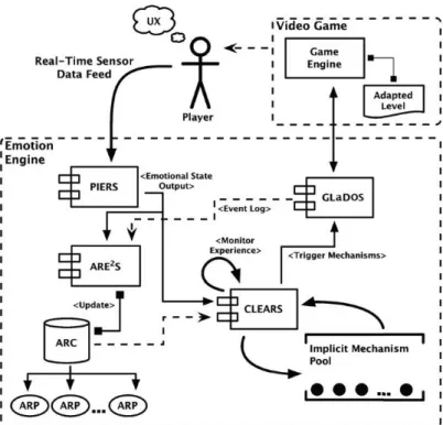
Figure 1: The Emotion Engine (E2) architecture. ... 8

Figure 2: Screenshot of a creature encounter event on a Vanish gameplay session publicly available on Youtube ...10

Figure 3: Representation of one of the plots used to readjust outliers ...12

Figure 4: Representation of one model in the 3D Space. ...19

Figure 5: Final Clustering Result ...22

Figure 6: SSE and Dispersion over Number of Clusters ...24

Figure 7: Sample of GODx emotional experience representation ...33

Figure 8: Fitness over time Comparison ...39

Figure 9: Arousal over time Comparison ...40

Figure 10: Arousal Difference ...44

Figure 11: Valence Difference ...45

Figure 12: Arousal Mean over time ...46

Figure 13: Arousal Mean Difference over time ...46

(16)

(17)

xvii

List of Tables

Table 1: Global Dataset Statistics ...12

Table 2: Global RMSE Values ...13

Table 3: Global Pearson Coefficient Values ...13

Table 4: RMSE Values ...14

Table 5: Average Number of Features ...14

Table 6: Ordered Features Usage When Classifying dA ...15

Table 7: Ordered Features Usage When Classifying dV ...16

Table 8: RMSE Global Value When Classifying dA ...17

Table 9: RMSE Global Values When Classifying dV ...17

Table 10: RMSE Global Values for Best Classifier ...17

Table 11: Coefficient of Determination Values ...19

Table 12: RMSE over Feature Segmentation ...26

Table 13: Features Usage over FSA ...27

Table 14: RMSE over FSA and Feature Segmentation ...27

Table 15: FSA over Demographic Segmentation ...27

Table 16: Top 5 Selected Features ...28

Table 17: Top 5 Globally Selected Features ...28

Table 18: RMSE over Classifiers ...29

Table 19: Classes RMSE over Demographic Segmentations...30

Table 20: NBF Experience Improvements along sorted PV's ...38

Table 21: Fitness Comparison ...43

(18)

(19)

xix

Abbreviations

Ai Initial Arousal - E{𝑟_𝐴}

BF BestFirst

BVP Blood Volume Pressure dA Delta Arousal - ∇𝐴 dV Delta Valence - ∇𝑉 ECG Electroencardiography EMG Electromyography

ER-IBF Emotional Regulated Indirect Biofeedback GODx Game Optimal Design Experience

GS Genetic Search IBF Indirect Biofeedback LFS Linear Forward Search LR Linear Regression

M5P M5 Model Trees and Rules MLP Multilayer Perceptron NBF Non Biofeedback NN Neural Network PV Parameter Values RS Random Search RSP Respiration

Vi Initial Valence - E{𝑟_𝑉} SC Skin Conductance SD Standard Deviation

(20)

(21)

Chapter 1

Introduction

Over the years, videogames have propelled innumerous breakthroughs in various fields - computer graphics, artificial intelligence, interaction techniques, physics simulation to name a few. These advances arose from the need of a more realistic game experience, reflected itself on better scenarios, more believable artificial behavior, incredibly realistic audio-visual effects and several other factors that bring to the player an ever growing level of immersion.

A wide range of emotions can arise from the act of playing a game. Players may become sad with a beloved character’s death, relieved with the ending of a confrontation, scared with the sound of a distant creature or even frustrated with repeated defeat. This subjective experience has its inception on the game designers that aim to convey to the player these desired emotions and experiences through the act of playing a game.

1.1 Context

Nowadays, gaming industry has been slowing shifting its focus from the technological department, and invested its resources on underexplored areas of gameplay experience. The search for the reasons that lead people to play (Ryan, Rigby, & Przybylski, 2006) and why it is a pleasurable experience (Ermi & Mäyrä, 2005) are subjects that have been vastly studied over the years. A converging thought has been presented many times: video games must provide an engrossing experience, taking the player from the real world and plunging him into the virtual world. Understanding and improving on this immersion is the key to produce better gaming experiences.

Although a fuzzy subject, immersion has been vastly referred to as the degree of envelopment the user has established with the virtual world. How “detached” he has become from

(22)

Introduction

2

the real world and believes he is in the virtual world (Jennett et al., 2008). How captivating a particular challenge is and how much emotion certain events arouse in the player.

1.2 Motivation and Objectives

The search for better levels of user experience (UX), lead to the potential use of Affective Computing and the detection of emotions on players. Ways to use these perceived emotions in-game to make the best possible experience to the player is of utmost relevance. The prediction of players’ behavior and emotional reaction can give game developers the tools to create much more immersive and entertaining experiences. It provides a way of assessing if the user experience of the target audience is the one game designers intended when creating the game. Even adaptive games can be vastly improved if the content generated in real-time takes into account the current emotional state of the player.

The primary objectives of this work are: obtain a dataset for the extraction of emotional results, Creation of players’ affective reaction models to a pre-determined number of events and the creation of a medium/high level simulator where the previously created models are used to identify the ideal game parameters (possible incorporation of real-time mechanisms).

1.3 Dissertation Structure

Beyond this introduction, this dissertation contains 5 more chapters. In chapter 2, the state of the art is described and related works are presented. In chapter 3, the affective reaction models are constructed and validated. In chapter 4, a possible correlation between physiological/demographic data and reported game experience. Chapter 5 consists the global scope of the work is detailed and explained. The last chapter presents a global overview and some conclusions of the work done.

(23)

Chapter 2

State of the Art

In this chapter, the state of the art is described and related works are presented in order to showcase what exists in the same domain and what are the problems faced. Section 2.1 will present current methods of emotional recognition through psychophysiological data. Subsequently, several works regarding the modelling of players’ experience are presented. Afterwards, the subject of affective gaming is discussed, in order to show how to augment players’ gaming experiences. We conclude the chapter with some final remarks.

2.1 Psychophysiological Emotion Detection

Recognizing human emotions through the study of physiological data is a subject that has been researched numerous times. The investigation of physiologically-controlled biofeedback techniques for gaming purposes dates back to late 1970s and early 1980s (Stern, R., Ray, W., & Quigley, 2000). In fact, physiological metrics seem to be the most popular choice, possibly due to their nature that allows the collection of continuous and unbiased data. One of the early works is “The Atari Mindlink”, an unreleased device that allowed to map traditional controllers using the users’ forehead muscles. The Japanese version of the title Tetris 64, released in 1998 for the Nintendo 64, included a biosensor that would change the game speed based on the user’s heart rate. Overall, these systems failed to achieve a better gaming experience and were seen as simple technological demonstrations. In the last decade however, the industry has shown a growing interest in the use of physiological signals to improve gamers’ immersion and experience (Kalyn, Mandryk, & Nacke, 2011).

A vast number of successful attempts have been made in the field of emotion recognition using physiological metrics. For instance (Haag, Goronzy, Schaich, & Williams, 2004) have

(24)

State of the Art

4

proposed that emotional states represented in the circumplex model presented by (Posner, Russell, & Peterson, 2005) can be modelled through Electromyography (EMG), Skin Conductance (SC), skin temperature, blood volume pressure (BVP), electroencephalographic (ECG) and respiration (RSP) sensors, reporting an accuracy of about 63% for valence and 89% for arousal (with a 10% error margin). A Neural Network (NN) classifier was used to predict both classes. Applying a similar NN classifier, research by (Leon, Clarke, Callaghan, & Sepulveda, 2007) has discretized valence in three different levels obtaining a recognition level of 71.4%. It uses Heart Rate (HR), BVP, Skin Resistance (SR) and two additional estimated parameters, the time gradient of SR (GSR) and its’ derivative. (Drachen & Nacke, 2010) showed that features extracted from SC and HR measures are highly correlated with the reported affection ratings obtained through a seven dimension In-Game Experience Questionnaire (iGEQ). On a similar note, (G. Yannakakis & Hallam, 2008) presented proof of correlation between BVP, HR and SC measures and high-level concepts such as “fun” in a game environment. A later study by (Martínez, Garbarino, & Yannakakis, 2011) reported that with only measures of HR and SC, they were able to predict affective states across games of different genres and dissimilar game mechanics.

Works on possible real-time recognition of emotion have also emerged (Mandryk & Atkins, 2007; Nogueira, Rodrigues, Oliveira, & Nacke, 2013a, 2013b). These take into consideration the possibility of a real world scenario usage. In order to provide continuous classification of a persons’ emotional state, a low computational cost is necessary. Furthermore, the usage of a small number of sensors is desirable to assist in their insertion during real gameplay.

2.2 Player Modelling

Parallel to biofeedback related emotion detection techniques, some research points to other ways to model player experience (G. N. Yannakakis & Togelius, 2011). The most direct and simple way is to ask the subjects themselves and build a model based on this data. Although this process may create very accurate models (Georgios N. Yannakakis, 2009), the human factor can lead to some problems. The vast presence of experimental noise (derived from human error in self-judgment, memory, etc.), the intrusiveness of the method among other factors can lead to some difficulty to analyze the data. Works such as (Tognetti, Garbarino, Bonarini, & Matteucci, 2010), have shown how self-reports can be successfully used to capture aspects of player experience. Other works on this area also model the users’ experience on an emotional basis (Shaker, Yannakakis, & Togelius, 2009). By observing crowd-sourced playing styles and features of level design, models were constructed that predicted player experience on different emotional dimensions: fun, challenge and frustration. Posterior work on the same data (Pedersen, 2010) added three more dimensions to the prediction. Although these models provide some insight to a players’ affective state, the low granularity of dimensions involved does not allow to capture all

(25)

State of the Art

5

the nuances of human emotions and affection. A less diffuse way to describe the emotional state of the player is desired.

Another existent method, is the use of gameplay data to try and build these models. The main assumption is that player actions and real-time preferences are linked to player experience, making possible the inferring of the player’s emotional state by studying patterns of the interaction (Conati, 2002; Gratch & Marsella, 2005). This method is the least intrusive one, becoming a candid possibility to real world usage. However as (G. N. Yannakakis & Togelius, 2011) state, the models are often based on several strong assumptions that relate player experience to gameplay actions and preferences, resulting in a low-resolution model of playing experience and its affective component.

(Leite & Pereira, 2010) exhibited a social robot that could recognize the user’s affective state and display empathic behavior. The users’ affective state is inferred through the current state of the game and interpreted according to an empathic behavior model. Complex game aspects such as storyline have also been shown to be dynamically adaptable to individual players, in such a way that a pre-determined reaction is achieved. (Figueiredo & Paiva, 2010) described a small study where by using an expert source manipulation, were able to dynamically adapt the storyline to the player, making him follow a pre-determined path. (Bidarra, 2013) based on actions performed by the player, and created classes of players with different characteristics.

Moreover, solutions that try to combine the previous forms are also frequent, resulting on a hybrid-approach. (Pedersen, 2010; Shaker et al., 2009) implemented gameplay and subjective player emotion models.

The presented work also uses a hybrid approach, using both psychophysiological data and subjective player emotion models. With this method we believe a more effective solution for modelling player experience is created.

2.3 Affective Gaming

The previous topics discussed the works done to detect and predict the affective reaction experienced by the players when playing a game. However, to create more engaging and overall better gaming experiences, changes to the actual game must be made. Having as basis the players’ models discussed, it becomes possible to use a player’s current emotional state to manipulate gameplay, corresponding to a new form of gameplay, presented by (Gilleade, Dix, & Allanson, 2005) as “Affective Gaming”. This process of improving game design is done by shifting the focus from static games with fixed contents to more dynamic systems. The presence of player models in game development allows the game developers to do just that, make informed decisions to elicit the desired emotions and affections on the player. The challenge resides in being able to model player behaviors and experiences and adapt the games’ content accordingly (Bidarra, 2013).

(26)

State of the Art

6

One of the early demonstrations of game enhancement (Bersak, McDarby, & Augenblick, 2001) presented a two-player competitive game where the speed of the avatar (dragon) is controlled by the users’ relaxation levels, measured through GSR. The more relaxed the user is, the faster the dragon becomes. This seems a common biofeedback game by mapping input controls to physiological data. However, the way the implementation was done counters this. By making the dragon speed increase when the player is relaxed and due to the competitive side of the game, players that became aroused started to lose, and because they were losing, they became even more aroused. By adapting itself to the players’ state, it falls on the “Affective Gaming” category. Yet, the moment the user becomes able to control their physiological data to influence the game outcome, the game transforms into a simple biofeedback game (Gilleade et al., 2005).

A significant work on the matter of affective gaming was presented by (Dekker & Champion, 2007). In it several subjects played a modified version of Half-Life 2 on a survival and horror based level. The difference to the original version was that, during gameplay, the game was dynamically modified by the player’s biometric information in an attempt to increase the “horror” experience. These changes reflected on audiovisual changes: dynamic changes in the game shaders, screen shake, dynamic changes in the background music, heartbeat sounds among others; and gameplay changes: new zombie spawning points, ‘bullet time’ effects, weapon damage, stealth mode etc. The results were encouraging, a vast majority of subjects liked the biometric-driven events, and nearly all of them acknowledged their potential.

More recent works have been done at Valve, (Ambinder, 2011) has presented several experiments using a players’ physiological data. One of them consisted of a mod to the popular title “Alien Swarm”, a top-down, team-based action shooter. The procedure was to index the players’ arousal, measured through SC levels, to the countdown timer. When high levels of arousal where detected, the timer speeds up. This created a more frenetic experience, raising even further the arousal levels, similar to (Bersak et al., 2001) experiment. Another experience tried to gain a rudimental understanding of the players’ affective reactions. By modifying the Left 4 Dead 2 AI Director. The AI Director is responsible for creating dynamic and variable experience by modifying game events, enemy spawns, health and weapon placement, boss appearances, etc. By determining the in-game encounters based on estimated arousal levels instead of predicted ones, greater values of enjoyment were reported. This lead to some insight into events which elicit enjoyment. In this work, an intriguing question was posed, “Can we determine optimal arousal patterns? “, “do we know the best way to model the players’ affective states?” (Kalyn et al., 2011) presented a mixed-methods study to discover the best use for direct (user controllable) and indirect (hard to influence) physiological control in games. It had a basis on a side-scrolling platform shooter game that used a traditional game controller as primary input. Via physiological sensors, the traditional interaction was augmented. Participants played with three combinations of physiological and traditional input. As (Nijholt & Tan, 2007) showed, satisfaction was reported by players out of learning to control their biofeedback through indirect physiological control. Moreover, the physiological augmentation of the game controllers provided a more fun

(27)

State of the Art

7

experience. A clear distinction was made by direct and indirect signals, players’ reported that physiological controls worked most effectively and were most enjoyable when they were appropriately mapped to game mechanics. On the other hand, indirect control was perceived as best used as a dramatic device in games to influence features altering the game world. Similar methods to shape players’ affective experience are presented by (Nogueira, 2013). In it, the adaptive design has its basis on a set of target emotional states and the usage of their emotional reactions to game events.

The design of affective games has also been a target of some approaches. (Gilleade et al., 2005) presented an approach to game design based on high-level design heuristics: assist me, challenge me and emote me (ACE). These can be used to create several different gaming experiences. ‘Assist me’ proposed a solution to players’ frustration (arising from missing clues, inability to advance due to difficulty, etc.) by measuring it using physiology signals and, combined with knowledge of the game context, provide mechanisms to identify this situation and adjust the game itself accordingly. Results gathered from their own affective game showed that casual gamers were the most sensitive to these changes. ‘Challenge me’ had its inception due to the difficulty provided by commercial games. Usually only three or more levels (easy, medium, hard) are presented and it is the user himself that indicates their perceived expertise, hoping it matched the game designers intent. This leads to inefficient challenges presented and subsequent lack of engagement. The solution is to dynamically alter the challenge provided by the game based on the user’s arousal, thus creating a more personalized gameplay experience. ‘Emote me’ refers to the emotional experiences players’ are provided with and the best way to deliver them. By determining the current users’ emotional state, and the intended one by the game designers, the game must modify its content to provoke the desired emotions.

Adding to the previous work, (Hudlicka, 2009) suggested a set of requirements for an affective game engine, with the purpose of allowing game developers the creation of better affective games. It presents a series of high-level requirements, not specifying their exact implementation. One of the central elements of this engine would be a knowledge-base that would contain information about emotions in general (their generation, influences, expression), and a depiction of the players’ and other non-playing-characters’ affective states. Four components with different functionalities would then be built that shared and changed this database: the recognition of the players’ emotion, the expression of emotions by both the player avatar and the game characters, the dynamic construction and maintenance of the players’ affective model (affective user models), and the modeling of emotion within the games’ characters (Hudlicka, 2008).

Lastly, (Nogueira & Rodrigues, 2013) proposed an implementation of these high-level abstract requirements through a psychophysiological approach nicknamed Emotion Engine (𝐸2₎

(28)

State of the Art

8

2.4 Summary

Over the years, the usage of both direct and indirect biofeedback in games has gained increased attention of researchers. Real time psychophysiological data provides several possibilities for improving gaming experience, whether being new ways of input or enhancing immersion levels via affective gaming. Our goal is to extend current work on the field by presenting a way to create affective reaction models from this psychophysiological data and use them to enhance gaming experiences, through the use of adaptive and parameterisable affective gaming. In addition, previous publications made by the author to some renowned journals present some relevant information (Nogueira, Aguiar, Rodrigues, & Oliveira, 2014a, 2014b).

(29)

Chapter 3

Affective Reaction Models

One of the main aims of this work is to create individual player models for the prediction of their respective emotional responses to a predetermined set of game events. This means that for each subject, given an initial emotional state and game event, their emotional reaction in both arousal and valence dimensions is predicted. As such, these models should obey Equation 1:

𝜙: ⋀𝑋Ω →𝑤⃗⃗

Where Λ is the set of possible emotional states and Ω the set of possible events. Thus, function Φ receives an emotional state λ, such that λ ∈ Λ and an event ϖ, such that ϖ ∈ Ω, and outputs a vector 𝑤⃗⃗ that contains the emotional reaction. This vector can have several dimensions, being their total number defined by the space used to define an emotional state. This work uses the circumplex model of affect as presented by (Posner et al., 2005). This space has two dimensions, Arousal and Valence. Valence depicts the nature of an emotion, lower values mean sadder emotions, higher values happier emotions. Arousal measures the level of excitement, how stron is the emotion. As such, the above vectors present some constraints.

∀ 𝑞 ∈ [1,2]: 𝑤⃗⃗⃗⃗⃗ ∈ [0, 10] 𝑞

3.1 Emotional Reactions Feature Extraction

For the creation of these affective emotional reaction models, an extraction of real-world emotional reactions was performed. In this study, these were extracted from 72 gameplay sessions of an indie horror game denominated Vanish. A total of 24 participants were present throughout this experience.

(30)

Affective Reaction Models

10

Vanish is a survival horror videogame where the player must escape a series of tunnels. This network of maze-like tunnels is procedurally generated. In order to escape, a series of key items must first be found and picked up by the player, only then being allowed to escape. At gameplay-time, a monstrous creature stalks and preys on the player, forcing him to avoid her at all costs. Several events happen in-game, both visual and audio, in an attempt to engage and involve the player in the game’s atmosphere. These events range from lights failing, pipes bursting or even the creature’s distant howl/cries. All these events, along with death, the locating of new items and creature encounters are tracked and constitute the whole set of considered game events.

As previously mentioned, the collected dataset originated from 24 players over 72 gameplay sessions. Regarding the subjects, they were randomly selected from a pool of interested candidates (N=89) being that their ages varied between 19 and 28 years old (µ = 22.47, σ = 2.50). The physiological data was obtained via a range of sensors: Skin Conductance, Heart Rate and facial EMG. Although an hybrid approach of the work was used, a more in-depth analysis of the process of mapping physiological input to emotional states can be found in (Nogueira, Rodrigues, et al., 2013a) combined with rules suggested by (Mandryk & Atkins, 2007). Regarding the special placement of these sensors, HR was derived from BVP, SC was measured at the players’ index and middle finger using two Ag/AgCL surface sensors snapped to two Velcro straps and facial EMG was measured at the zygomaticus major (cheek) and the corrugator supercilii (brow) muscles.

This physiological data is then processed, producing a 1:1 both arousal and valence ratings, being afterwards segmented by study participant. The automatically generated timestamps were then synchronized to these AV ratings in order to extract an emotional response. Singular emotional reactions were then extracted by using a time window of 0.5 seconds prior and 5

Figure 2: Screenshot of a creature encounter event on a Vanish gameplay session publicly available on Youtube

(31)

11

seconds after the correspondent timestamp. The contextualization of the players’ immediate emotional response prior to occurrence of the game event and the analysis of his emotional reaction is possible due to this time window. Note that these values were not random, they are based on the detected physiological data and player perception delays of game events (Nogueira, Torres, & Rodrigues, 2013).

Additionally, a total of twelve features are extracted for each emotional reaction: six related to arousal and another six pertaining to valence levels. Both valence and arousal share the same feature extraction process. Onwards from the gameplay event timestamp, the following features are created:

- 𝐸{𝑟}: Initial value, calculated as the average of the maximum and minimum values registered in the 0.5 seconds prior to the game event

𝑎𝑣𝑔(𝑚𝑎𝑥{𝑟}, 𝑚𝑖𝑛{𝑟}) - 𝜇{𝑟}: Mean of the signal

- 𝜎{𝑟}: Standard Deviation of the signal - 𝑀{𝑟}: Maximum Value of the signal - 𝑚{𝑟}: Minimum Value of the signal

- 𝐷ℎ: Absolute time period between minimum and maximum value

𝐷ℎ= | 𝑡𝑚𝑎𝑥ℎ {𝑟} − 𝑡𝑚𝑖𝑛ℎ {𝑟} |

- ℎ𝑖𝑛{𝑟}, ℎ𝑜𝑢𝑡{𝑟} 𝑎𝑛𝑑 ℎ𝑒𝑣{𝑟}: Auxiliary features denoting the reactions beginning,

ending and event timestamps.

The delta value of the reactions (ΔA , ΔV) are calculated as the greatest difference registered between the maximum and minimum values of the initial time window frame (0.5 seconds prior to the game event), and the maximum and minimum values of the remaining event time window. Over 1400 (fourteen hundred) individual emotional reactions were recorded. However, a more in depth analysis to this data brought some questions to the surface.

First of all, one particular subject presented a greatly reduced number of events and emotional reactions. Moreover, nearly all of his emotional reactions were concentrated on a pair of events, resulting in insufficient data when looking at the full spectrum. As such, this subject has been completely removed from subsequent phases. Additionally, two subjects didn’t have their emotional reactions recorded due to hardware failures making impossible their inclusion.

Lastly, a total of three events were not present in more than half of the input data, and were, as such, entirely eliminated from the dataset. Their presence would wrongly inflate the classifiers’ performance. After all this filtering process, of both subjects and events, over 1160 emotional reactions are present in the full dataset.

An additional manual examination was made to the data. For each pair of subject and event, their emotional reactions were drawn along the initial arousal and valence values. This allowed to perceive outliers, possibly originated from another event that occurred at the same time. Only values that were vastly irregular with the other data were adjusted. These adjustments still preserved some of this point disparity, however their value was changed to better represent the

(32)

12

overall players’ response. This was done to preserve the maximum amount of information and because the detection of real outliers is a complex and difficult decision.

A general overview of the statistics of the final dataset is present in Table 1. To note that 𝐴𝑖 ≡ E{𝑟𝐴}, 𝑉𝑖 ≡ E{𝑟𝑉}, 𝑑𝐴 ≡ ∇𝐴, 𝑑𝑉 ≡ ∇𝑉 (see abbreviations)

Mean Median Standard Deviation

Ai 6,4296 8,6054 0,6844

Vi 4,3369 5,8750 0,5520

dA 0,2388 0,2342 0,2168

dV 0,3356 0,3142 0,3226

Table 1: Global Dataset Statistics

As is easily noted, the average initial arousal level is larger than the baseline value (5), while its valence counterpart shows a lower value. This is probably due to the games nature. Being a horror game, players remain in a constant state of alert.

3.2 Machine Learning

One of the most fundamental steps of this thesis is the creation of affective reaction models. The ability to predict the players’ emotional responses is of utmost importance and relevance.

The first approach to the creation of these affective reaction models is the employment of machine learning. With this, a model is created that predicts the emotional response of a subject to a certain event along all emotional states spectrum. This whole process was segmented into several phases, namely: single classifiers, optimal feature selection algorithm and lastly the creation of these models.

(33)

13

3.2.1 Single Classifiers

To serve as a baseline and due to the exploratory nature of this work, the first models created used a single feature. This can lead to some conclusions and deductions that might prove valuable in later phases. Possible correlations between features and classes can also be discovered through this approach.

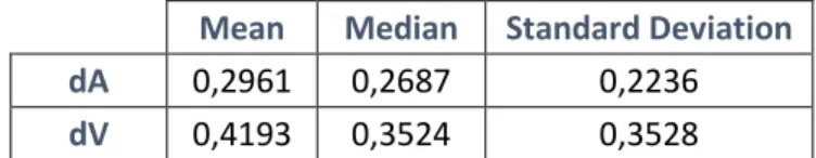
Mean Median Standard Deviation

dA 0,2961 0,2687 0,2236

dV 0,4193 0,3524 0,3528

Table 2: Global RMSE Values

Mean Median Standard Deviation

dA 0,5307 0,5444 0,4061

dV 0,5453 0,5675 0,3967

Table 3: Global Pearson Coefficient Values

Root Mean Squared Error (RMSE) gives us a solid way to evaluate the dimensionality of the errors involved in the classification. Moreover, due to its nature it penalizes the existence of very strong outliers, which is something beneficial viewing that large errors in classification can lead to extremely bad results later on. As one can see in Table 2, the error values presented are very large taking into consideration the range of values in the classes involved. These error rates are significantly larger than the original Standard Deviation, leading to the belief that the classification has poor results. Also note the vastly superior error rates in the Valence dimension. Both an increase in Mean error and its Standard Deviation is noticeable. This probably originates from lower volatility in estimating arousal, opposed to valence, as shown in (Nogueira, Rodrigues, et al., 2013a).

The same can be seen in the Pearson Correlation Coefficient presented in Table 3. This value, ranging from minus one to one, measures the linear correlation between variables, higher absolute values representing higher correlations. As one can see, the mean values presented are relatively small. Furthermore, the Standard Deviation is extremely large, indicating abnormal classifications throughout.

A closer look to the detailed RMSE values showed that Arousal related features provided less error values. The same happened in the Valence dimension. However, this difference is very small, not providing sufficient insight.

(34)

14

3.2.2 Optimal Feature Selection Algorithm

Because the classifying/regression approach is dependent on the features selected to create it, the selection of these features can vastly improve the viability of the models. As such, several feature search methods are tested to improve the overall results. Because of its proven reliability and results, the attribute evaluator used can be seen in (Hall, 1999). A total of four different search methods are employed, Best First (BF), Random Search (RS), Linear Forward Selection (LFS) and Genetic Search (GS). The RS method serves as baseline due to its random nature. The last ones are well accepted among the industry and have proven their values by having good results over a vast selection of fields and applications. Several other search methods were not used due to some constraints, some required an evaluator function that only deals with single features excluding subsets of features (similar to previous phase). Others, for example Exhaustive Search, required too much processing power, making them undesirable.

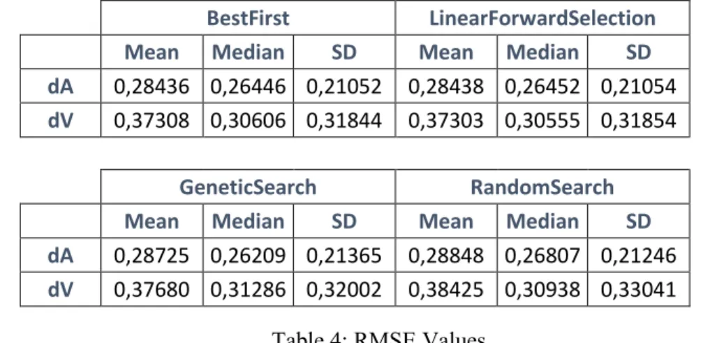
Each of the search methods used is then combined with three different classifiers (the reason for the usage of these classifiers is presented later) and are evaluated. The results obtained are shown in Tables 4 through 7:

BestFirst LinearForwardSelection Mean Median SD Mean Median SD dA 0,28436 0,26446 0,21052 0,28438 0,26452 0,21054

dV 0,37308 0,30606 0,31844 0,37303 0,30555 0,31854

GeneticSearch RandomSearch Mean Median SD Mean Median SD dA 0,28725 0,26209 0,21365 0,28848 0,26807 0,21246

dV 0,37680 0,31286 0,32002 0,38425 0,30938 0,33041 Table 4: RMSE Values

BestFirst GeneticSearch LinearForwardSelection RandomSearch

dA 2,11934 3,09053 2,11934 4,02058

dV 2,13580 3,06584 2,13580 4,11523

Total 2,12757 3,07819 2,12757 4,06790 Table 5: Average Number of Features

(35)

15

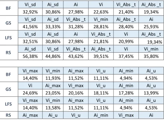
BF Ai_sd Ai Vi_sd Ai_Abs _t Vi_Abs _t Vi_max

36,21% 30,86% 30,04% 22,22% 20,58% 14,40%

GS Ai_sd Vi_sd Vi_Abs _t Ai_Abs _t Ai Ai_max

37,45% 37,04% 32,10% 30,04% 29,22% 23,46%

LFS Ai_sd Ai Vi_sd Ai_Abs _t Vi_Abs _t Vi_max

36,21% 30,86% 30,04% 21,40% 20,99% 14,40%

RS Ai_sd Vi_sd Ai_Abs _t Vi_Abs _t Ai_u Ai_max

51,03% 45,27% 41,15% 40,74% 35,80% 30,45%

BF Ai_max Vi Ai_u Ai_min Vi_u Vi_min

11,93% 11,52% 9,05% 8,64% 8,23% 8,23%

GS Vi_min Ai_u Ai_min Vi Vi_max Vi_u

23,05% 22,63% 21,81% 19,75% 19,34% 13,17%

LFS Ai_max Vi_min Ai_u Vi Ai_min Vi_u

11,93% 11,52% 9,05% 9,05% 8,64% 7,82%

RS Vi_min Ai_min Vi Ai Vi_max Vi_u

30,04% 27,16% 26,75% 25,51% 25,10% 23,05% Table 6: Ordered Features Usage When Classifying dA

BF Vi_sd Ai_sd Ai Vi Vi_Abs _t Ai_Abs _t

32,92% 30,86% 27,98% 22,63% 21,40% 19,34%

GS Vi_sd Ai_sd Vi_Abs _t Vi_min Ai_Abs _t Ai

41,56% 33,33% 31,28% 28,81% 28,40% 25,93%

LFS Vi_sd Ai_sd Ai Vi_Abs _t Vi Ai_Abs _t

32,51% 30,86% 27,98% 21,81% 20,99% 19,34%

RS Ai_sd Vi_sd Vi_Abs _t Ai_Abs _t Vi Vi_min

56,38% 44,86% 43,62% 39,51% 37,45% 35,80%

BF Vi_max Vi_min Ai_max Vi_u Ai_min Ai_u

14,40% 11,93% 11,52% 11,11% 4,94% 4,53%

GS Vi Ai_max Vi_max Vi_u Ai_min Ai_u

24,69% 23,05% 20,16% 18,11% 17,28% 13,99%

LFS Vi_max Vi_min Ai_max Vi_u Ai_min Ai_u

14,40% 13,58% 11,52% 11,11% 4,94% 4,53%

(36)

16

29,63% 28,40% 27,16% 25,10% 23,05% 20,58% Table 7: Ordered Features Usage When Classifying dV

Analysis of the Global RMSE values on this approach bring forth some conclusions (Table 4). First, the use of FSA over Single Feature decreases the error value significantly. This means the usage of a subset of features over a single feature brings visible benefits. Second, Random Search has, as expected, the largest error. This is due to the random nature of the method. However, Genetic Search presents marginally better results. Best First and Linear Forward Selection have the lowest error values. They present similar and largely better results.

Table 5 presents the average number of features used by each FSA when trying to classify each dimension. A similar pattern is seen. Random Search uses approximately four features model, while LFS and BF only half. Genetic Search sits on the middle of this table. Some ratings can already be made to these FSA. Random Search has the highest error value and uses the most features. Next comes Genetic Search with better results. BF and LFS present similar results and expressively better than their counterparts. Because of this BF is the FSA used in posterior phases. On Table 6 and Table 7 the usage of features per FSA is depicted. The presented ordered list allows for a quick inspection to the most used features to predict both dimensions. Similar to the single feature results, Arousal features tend to be chosen more often when classifying the emotional reaction in the Arousal dimension. The same phenomenon is manifested in the Valence dimension.

3.2.3 Model Creation

The final step is the creation of the models using the feature selection algorithm previously chosen. Viewing that this is a regression problem, several classifiers can be used to predict these emotional reactions. However due to some previous observations, only three classifiers were chosen. This relates to some of the patterns discovered in the previous phases, during the pre-processing of the data. In general, two strong patterns emerged from the visualization of the data, a linear model and a more quadratic and complex type. For this reason, three different classifiers were used and their results compared in order to obtain the best prediction: Linear Regression (LR), M5 Model Trees and Rules (M5P) and Multilayer Perceptron (MLP). Both the M5P and the MLP classifiers can easily handle complex behaviours. However, the last one can more easily fall in the pit of over fitting. Nevertheless, both are tested to ensure the best possible result. For each one of these three classifiers, a total of three evaluation modes are presented. Presented in order of preference: 10-fold cross-validation, 3-fold cross validation and the use of the whole testing set for training. Some key results are shown in Tables 8, 9 and 10:

(37)

Affective Reaction Models 17 Average SD LR 0,311353 0,075435 M5P 0,29591 0,067145 MLP 0,238855 0,093251

Table 8: RMSE Global Value When Classifying dA

Average SD LR 0,400987 0,138804

M5P 0,396201 0,127097

MLP 0,323791 0,139332

Table 9: RMSE Global Values When Classifying dV

Average SD dA 0,230942 0,080196

dV 0,312054 0,123437

Table 10: RMSE Global Values for Best Classifier

As is seen in Table 8 and Table 9, a large difference exists in the error rates between classifiers. Linear Regression presents the worst results, with both high average and standard deviation error values. On the other hand, M5P shows better results. However, only a small decrease in error is seen. The decrease in the Standard Deviation of the errors’ values is an encouraging result. Even so, it is still not a satisfactory solution. Moreover, due to the MP5 ability to mimic the LR and create more complex “functions”, this increase in performance was expected. The Multilayer Perceptron classifier showcases largely better results. A vast difference in the average error is seen. However, the large increase in the Standard Deviation values brings suspicion to the validity of this solution. Overfitting may have occurred.

As a final global overview, the RMSE values when the same and best classifier per event is used are shown in Table 10. This approach makes the posterior comparison between subjects possible by making each related model based on the same classifier. Nevertheless, although the results are slightly better than previous ones, when looking at the global scope they are not adequate enough. Error rates are in the same magnitude as the Standard Deviation for the class in question, making the results not very positive.

(38)

18

3.3 Clustering Approach

The previous machine learning approach treated individuals as single entities, without any relation between them. A classifier predicted the players’ affective reaction to an event based on the optimal subset of features. This however might not produce the best results. Viewing that we are modelling human behaviour, some patterns and relationships between subjects can help strengthen these predictions. As such, and with the intent of approximating the human world, a second approach was attempted where groups of people that present similar emotional responses are treated as whole. This is done via hierarchical clustering.

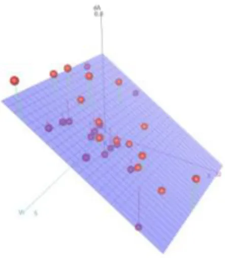
In order to make possible the comparison of models and their subsequent distances calculated, an initial stage of creating these models with the same domain is necessary. Only with these distances is the actual clustering possible. Due to some correlations presented between features and classes, the creation of these models was transformed into a three-dimensional space, with two of the axes representing the features used: initial arousal (Ai) and initial valence (Vi) and the third axis representing the expected emotional reaction in either arousal or valence levels (dA or dV) that the player experienced. The purpose is to find a relationship between the affective reaction (response variable) and the combination of the two features (predictors).

As in the previous approach, taking into consideration the perceived distributions of the reactions, the relationships were built through linear and non-linear regression models. Viewing that using an automatic approach to discover the regression model that produces better results will most certainly lead to overfitting and high-degree polynomials, a supervised approach was followed. After a manual analysis of a large number of these models, some conclusions were inferred. First, the regression models should not exceed a third degree polynomial. A bigger degree represents a negligible increase in the fitness of the model while showing a large increase in symptoms of overfitting. Lastly, due to the nature of a second degree polynomial, being characterized for its parabolic shape, the models created with this degree will present an ever growing emotional reaction either in positive or negative values. This is incongruent with common sense, which led to the decision of not using these models.

Ultimately, the regressions were produced using either linear or third degree regressions, depending on the number of points available for the model. Figure 4 illustrates a sample plot of a model. The upward axis represents the reaction. A Linear Regression is already present. Table 11 presents a small error analysis.

(39)

19

Average Standard Deviation

𝑹𝟐 Value 0,954267 0,208303

Adjusted 𝑹𝟐 Value 0,704619 0,509913 Table 11: Coefficients of Determination Values

Present in Table 11 are the coefficients of determination for the created models. The R-squared value ranges from zero to one, indicating how well data points fit a statistical model, in this case the regressions. A value of zero specifies that the model explains none of the variability of the response data around its mean. A value of one indicates all the variability is explained by the model. The adjusted R-squared is a modified version of R-squared that adjusts itself for the number of predictors in the model. The adjusted R-squared increases only if the new term improves the model more than would be expected by chance.

As can be seen, the R-squared value shows a very high average value with relatively small standard deviation. On the other hand, the adjusted R-squared variable presents a moderately smaller mean, with higher standard deviation. This relates to the low number of points present in the models. Due to the difficulties of retrieving a high number of emotional reactions already discussed earlier, the number of emotional reactions per model is not very high. Because of that, some models created present some overfitting as can be seen by the high R-squared value. Furthermore, because the models are built upon a low number of points, the adjusted R-squared value penalizes heavily the usage of linear and even more the quadratic models.

Each one of these models predicts the emotional response of one subject to a certain event over one dimension (either arousal or valence). As such, a total of 32 regression surfaces are created that describe an individual player’s emotional reactions over the AV emotional space. The

(40)

20

next step is to create a distance matrix that depicts the differences between emotional responses. For that to happen, these models need to be compared. This is done via the mapping of these models over all the AV space. The generation of a hyper-dimensional matrix that ranges from [0, 10] for both feature response variables (initial arousal and valence) with a 0.1 increment. By standardizing these models representations, they can easily be compared and their differences evaluated.

The next step is the creation of a distance matrix from which the hierarchical clustering is done. For that, a way to quantify the distance between the maps created is needed. The current implementation provides three different distance calculations and an extra post-processing stage that scaled these distances over several functions. Relatively to the distance calculations, the first one is a Euclidean distance.

This a well known measure for distance that has proved its usefulness in various fields. All points of the models are compared and the average Euclidean distance between points is then used as the distance between models. This procedure of calculating the distance between all the models’ points and then averaging this sum is used for all distance calculations.

The second calculation has its basis on an exponential distance function. This sanctions bigger distances even further, increasing their value. Additionally, similar models maintain a very low distance tightening their relationship.

Finally, the third method simply uses the normal distance, with no alteration to its original value. 𝐸𝑢𝑐𝑙𝑖𝑑𝑒𝑎𝑛 𝑑𝑖𝑠𝑡𝑎𝑛𝑐𝑒 = √∑(𝑃[𝑘] − 𝑀[𝑘])2 𝑛 𝑘=0 𝐸𝑥𝑝𝑜𝑛𝑒𝑛𝑡𝑖𝑎𝑙 𝑑𝑖𝑠𝑡𝑎𝑛𝑐𝑒 = ∑ e 𝑃[𝑘]−𝑀[𝑘] 𝑛 𝑘=0 𝑛 𝑁𝑜𝑟𝑚𝑎𝑙 𝑑𝑖𝑠𝑡𝑎𝑛𝑐𝑒 = ∑ 𝑃[𝑘] − 𝑀[𝑘] 𝑛 𝑘=0 𝑛 𝑛 = 𝑛𝑢𝑚𝑏𝑒𝑟 𝑜𝑓 𝑝𝑜𝑖𝑛𝑡𝑠 𝑖𝑛 𝑠𝑒𝑞𝑢𝑒𝑛𝑐𝑒 𝑃[𝑥] = 𝑣𝑎𝑙𝑢𝑒 𝑜𝑓 𝑠𝑒𝑞𝑢𝑒𝑛𝑐𝑒 𝑃 𝑖𝑛 𝑡ℎ𝑒 𝑝𝑜𝑖𝑛𝑡 𝑥

A post-processing stage was made. It was an experiment that tried to modify the whole range of distances calculated in order to see if it would yield better results. The general idea was to penalize certain ranges of distances, for example differences in the higher distance ranges are attenuated. Sigmoidal, logarithmical and the original linear functions were used. However, it was

(41)

21

later revealed that the original linear function produced better results, which led to no post-processing changes made in the final data.

At this stage, we have the tools to determine the distance between each pair of player/event regarding one emotional dimension. We need to correctly merge these values in order to create a distance between subjects. First, we create matrices holding the distances between subjects for a single game event over one emotional dimension. Since we have no evidence that any particular game event or emotional dimension has higher influence on the games’ affective experience, we can merge this “partial” distance matrices by averaging all their cells, assuming the correspondent cell orders are preserved. This brings forth a new global matrix holding the distances between subjects over all game events and emotional dimensions. With this new matrix, a hierarchical clustering algorithm can be applied to cluster players.

The hierarchical clustering used employed the Ward’s method (Joe H . Ward, 1963) for the criterion of choosing which clusters to merge, meaning the objective function is the error of sum of squares. Furthermore, a multi-scale bootstrap resampling process is used, allowing the assessment of uncertainty in this clustering approach. More specifically, Approximately Unbiased (AU) and Bootstrap Probability (BP) p-values are computed. Note however that the AU p-values, computed via multiscale bootstrap resampling, provide a better approximation to unbiased p-value than the BP p-value that is computed by normal bootstrap resampling. These p-values represent the confidence that a particular cluster is supported by the data, not simply caused by “sampling error” but may stably be observed if we increase the number of observations. As a more formal definition for these values, a cluster presenting an AU p-value of x has the null-hypothesis “the cluster does not exist” rejected with a significance level s = 100 – x. In sum, high AU p-values provide high confidence to the clusters found. With this in mind, all the results of the different distance matrices generated were manually analysed. The result was the selection of the exponential distance. The final result of this hierarchical clustering approach is presented in Figure 5.

(42)

22

As can be seen, the result presents high AU p-values throughout all the clusters found, leading us to the belief of a solid global solution. Moreover, the clusters seem well distributed, fact that can probably be attributed to the different demographics used in the extraction of the emotional responses.

As previously mentioned, the whole idea of this approach was to make the construction of the affective reaction models more congruent with the relations seen in human behavior, where several kind of people react similarly amongst themselves. As such, the choice of clustering relates to this fact. However, the final models work with a fixed set of clusters, whether they came from hierarchical or non-hierarchical clustering is irrelevant. The choice of hierarchical clustering relates to another fact. Because we have demographic information about the specific subjects in question, some analysis can be done relating the clusters and this information. Because of the way hierarchical clustering works, this can be done over all number of clusters. A clustering approach like for example x-means (k-means with automatic cluster number identification) would not preserve the clusters through the increase in the cluster numbers, disabling the possibility of studying this relationship. A manual observation was made regarding this issue, resulting in some encouraging results. Various clusters showed similar demographic information such as gender, type of gamer and the predisposition to horror games. Others presented correspondence in a

(43)

23

combination of several features. Note however that, due to time issues, not all cluster numbers were properly analyzed.

3.3.1 Clustering Validation

Although AU p-values computed via multiscale bootstrap resampling provide a good measure of the clusters strength, one more question remains. Viewing that a number of clusters needs to be determined in order to construct the models, a way to evaluate the “goodness” of the resulting clusters is needed to evaluate the several possible number of clusters. As such, two internal indexes are used to measure this: cluster cohesion and cluster separation.

Cluster cohesion measures how closely related objects in the same cluster are. It is the sum of the weight of all links within a cluster, calculated via the within cluster sum of squares. An average of all the clusters values is used to present a global value of cohesion.

Cluster dispersion quantifies the level of distinctiveness between clusters. It is the sum of the weight of all links within a cluster, measured by the between cluster sum of squares. The same procedure of averaging all the values from a particular cluster number is applied for the discovery of a global value. Note however that in the case of separation each cluster has associated N-1 measures, being N the number of clusters.

𝐶𝑜ℎ𝑒𝑠𝑖𝑜𝑛 = ∑ ∑ (𝑥 − 𝑚𝑖)2 𝑥∈𝐶𝑖 𝑖 𝐷𝑖𝑠𝑝𝑒𝑟𝑠𝑖𝑜𝑛 = ∑ |𝐶𝑖|(𝑚 − 𝑚𝑖)2 𝐶𝑖 = 𝐶𝑙𝑢𝑠𝑡𝑒𝑟 𝑖 |𝐶𝑖| = 𝑆𝑖𝑧𝑒 𝑜𝑓 𝐶𝑙𝑢𝑠𝑡𝑒𝑟 𝑖 𝑚𝑖 = 𝐶𝑒𝑛𝑡𝑟𝑜𝑖𝑑 𝑜𝑓 𝐶𝑙𝑢𝑠𝑡𝑒𝑟 𝑖

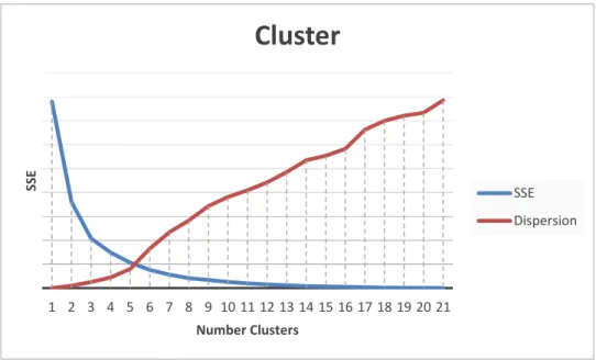
A representation of both these measures along the number of clusters can be seen in Table 6.

(44)

24

As seen in Figure 6, one can say the best number of clusters happens when the cohesion has low values and the separation high ones. However, as can be seen, these optimal values only happen at extremely high number of clusters, defeating the purpose of the clustering approach. As such, the best approach is to use the number of clusters that represent the best “gain” in both these dimensions comparatively to the previous number. This means we need to discover the number of clusters where the “acceleration” of the cohesion decreases and the “acceleration” of the separation increases. A simple way to tackle this is to integrate these values twice and inspect the local maximum and minimums. We are trying to find a minimum in cohesion, and a maximum in dispersion, representing a loss of efficiency when increasing the number of clusters. In the case of our clustering, the result obtained was 6 (six) as the best number of clusters.

After this number is calculated, the task of creating the various clusters’ affective reaction models is possible. With these models, the players’ individual ones can be easily represented as a composite of all the clusters models with different weights. These weights are related to the differences encountered between the original individual models and the clusters ones. The implementation finds the sum of all distances between one player and all the clusters and uses it to find all the weights.

𝑊𝑒𝑖𝑔ℎ𝑡𝑖,𝑘 = ∑ 𝑑𝑖𝑠𝑡𝑎𝑛𝑐𝑒𝑥 𝑖,𝑥 𝑑𝑖𝑠𝑡𝑎𝑛𝑐𝑒𝑖,𝑘 𝑊𝑒𝑖𝑔ℎ𝑡𝑖,𝑘 = 𝑤𝑒𝑖𝑔ℎ𝑡 𝑜𝑓 𝑐𝑙𝑢𝑠𝑡𝑒𝑟 𝐾 𝑖𝑛 𝑠𝑢𝑏𝑗𝑒𝑐𝑡 𝑖 𝑑𝑖𝑠𝑡𝑎𝑛𝑐𝑒𝑖,𝑘 = 𝑑𝑖𝑠𝑡𝑎𝑛𝑐𝑒 𝑜𝑓 𝑠𝑢𝑏𝑗𝑒𝑐𝑡 𝑖 𝑡𝑜 𝑐𝑙𝑢𝑠𝑡𝑒𝑟 𝐾 1 2 3 4 5 6 7 8 9 10 11 12 13 14 15 16 17 18 19 20 21 SSE Number Clusters

Cluster

SSE Dispersion

(45)

Demographic Study

25

Chapter 4

Demographic Study

To evaluate the relative impact of different types of Indirect Biofeedback (IBF) adaptation mechanics, the original extraction of the emotional reactions made the participants play three different versions of the game: two augmented using the biofeedback mechanics and one control condition. Each game version presented the same gameplay elements and mechanics. Both the game design and biofeedback adaptations were developed during an extended alpha-testing period using an iterative prototype over 3 months, gathering feedback from over 20 individuals not included in this study. After a brief description of the experiment and providing informed consent, players completed a demographics questionnaire. Participants also completed a game experience questionnaire (GEQ) (IJsselsteijn, Poels, & De Kort, 2008). Additionally, they were also asked to report their Fun ratings in a 10-point Likert scale. The full extracted features follow:

- Demographic Data

o GType - Reported Gamer Type: “Hardcore” or “Softcore” o Likes - Predisposition towards Horror Games: “Yes” or “No” o Gender - “Male” or “Female”

- Physiological Data

o SeqDur - Game Session Duration (min) o {X} - Arousal or Valence dimension o {X}Mean - Mean of the signal

o {X}SD – Standard Deviation of the signal o {X}P - Number of Absolute Peaks

o {X}PMin - Number of Peaks Per Min o {X}PInt – Average Peak Intensity o {X}PMag - Average Peak Magnitude o {X}Max – Maximum signal value o {X}Min – Minimum signal value - User Experience

(46)

Demographic Study 26 o Challenge (Chall) o Competence (Comp) o Flow (Flow) o Immersion (Imm) o Fun (Fun) o Tension (Ten)

In this section we aim to create computational models of user experience through the usage of demographic and physiological features. An optimal feature subset selection procedure capable of capturing non-linear relationships is employed. Finally, we use the optimal feature subset for each user experience dimension identified by the best-performing feature selection algorithm (FSA) - measured in terms of its achieved root-mean square error (RMSE) - to create computational models of user experience. All features are explored in this phase (physiological and non-physiological).

4.1 Single Model

The first step for the analysis of this data, is the creation of a single predicting model. Because the features include physiological and non- physiological data, three different feature subsets are used in order to further compare these two sources of information. One subset only contains biofeedback features, another only demographic ones, and the last one can contains both. This allows us to differentiate between demographic and physiological data for the classification of user experience. Additionally, the usage of all features can be seen as a baseline.

A global overview regarding the first phase where a single model was constructed follows:

Imm Ten Comp Chall Flow Fun Average All 1,682971 1,83367 2,54955 2,153161 2,025733 1,229042 1,912354

Bio 1,491728 1,859111 2,148719 1,949156 2,17748 1,273107 1,81655

Non-Bio 1,423103 1,52644 2,687004 1,905734 1,976445 0,989578 1,751384

Average 1,532601 1,73974 2,461758 2,002684 2,059886 1,163909 1,826763 Table 12: RMSE over Feature Segmentation

Likes SeqDur Sex Cond VPMin BestFirst 12 10 10 8 8

GeneticSearch 12 10 10 8 8

LinearForwardSelection 11 12 10 8 8

(47)

Demographic Study

27

Table 13: Features Usage over FSA

As show in Tables 12 and 13, the construction of the single model stems some large errors in certain related user experiences. However, “Fun” and “Immersion” reported low error values. Another deduction that can be made relates to the features. Nearly all classes presented smaller errors when the features used where only Demographic ones. Additionally, the FSAs’ vastly recognized this type of features as very valuable. This is probably the same situation seen in the Machine Learning approach in the construction of the affective reaction models, human nature leads to the existence of similar experiences between some groups of people. To tackle this problem, viewing that demographic data is available and presents better results, the whole population was segmented via these features. This means that instead of one single model for the prediction of a class, several ones are created, each one containing a demographic segmentation of the population, for example male players.

4.2 Feature Selection Algorithm

Some data retrieved regarding the several Feature Selection Algorithms follows:

BestFirst GeneticSearch LinearForwardSelection All 1,772586 1,803699 1,772586

Bio 1,762442 1,794179 1,762442

Non-Bio 1,694701 1,691236 1,694701 Table 14: RMSE over FSA and Feature Segmentation

BestFirst GeneticSearch LinearForwardSelection

Cond NB 2,178031 2,22728 2,178031 NV 1,723597 1,753616 1,723597 V 1,855355 1,949551 1,855355 GType Hard 1,451051 1,514739 1,451051 NA 1,461829 1,442075 1,461829 Soft 2,148233 2,079193 2,148233 Likes N 1,981011 2,085534 1,981011 Na 1,461829 1,442075 1,461829 Y 2,051743 2,01593 2,051743 Sex F 2,204128 2,299506 2,204128 M 1,572497 1,632421 1,572497

Affective Game Design: Creating Better Game Experiences based on Players' Affective Reaction Model

F

ACULDADE DE

E

NGENHARIA DA

U

NIVERSIDADE DO

P

ORTO

Affective Game Design:

Creating Better Game Experiences based

on Players’ Affective Reaction Model

Rúben Pinto Aguiar

Mestrado Integrado em Engenharia Informática e Computação

Supervisor: Prof. Rui Rodrigues (PhD)

Co-Supervisor: Pedro Nogueira (MSc)

Affective Game Design:

Creating Better Game Experiences based on Players’

Affective Reaction Model

Rúben Pinto Aguiar

Mestrado Integrado em Engenharia Informática e Computação

Aprovado em provas públicas pelo Júri:

Presidente: António Augusto de Sousa (Prof. Associado)

Vogal Externo: Pedro Miguel do Vale Moreira (Prof. Adjunto)

Orientador: Rui Pedro Amaral Rodrigues (Prof. Auxiliar Convidado)

____________________________________________________

Abstract

Resumo

Acknowledgements

Contents

List of Figures

List of Tables

Abbreviations

Chapter 1

Introduction

1.1 Context

1.2 Motivation and Objectives

1.3 Dissertation Structure

Chapter 2

State of the Art

2.1 Psychophysiological Emotion Detection

2.2 Player Modelling

2.3 Affective Gaming

2.4 Summary

Chapter 3

Affective Reaction Models

3.1 Emotional Reactions Feature Extraction

3.2 Machine Learning

3.2.1 Single Classifiers

3.2.2 Optimal Feature Selection Algorithm

3.2.3 Model Creation

3.3 Clustering Approach

3.3.1 Clustering Validation

Cluster

Chapter 4

Demographic Study

4.1 Single Model

4.2 Feature Selection Algorithm