Deep neural networks for image quality: a comparison study for identification photos

(1)

University Institute of Lisbon

Department of Information Science and Technology

Deep neural networks for image

quality: a comparison study for

identification photos

José Miguel Costa Ruivo

Dissertation in partial fulfillment of the requirements for the degree of

Master in Computer Science and Business Management

Supervisor

PhD, João Pedro Afonso Oliveira da Silva, Assistant Professor,

ISCTE-IUL

Co-supervisor

PhD, Maurício Breternitz, Invited Associate Professor, University of

Lisbon

(2)

(3)

Resumo

Muitas plataformas online permitem que os seus utilizadores façam upload de im-agens para o perfil das respetivas contas. O facto de um utilizador ser livre de submeter qualquer imagem do seu agrado para uma plataforma de universidade ou de emprego, pode resultar em ocorrências de casos onde as imagens de perfil não são adequadas ou profissionais nesses contextos. Outro problema associado à submissão de imagens para um perfil é que, mesmo que haja algum tipo de controlo sobre cada imagem submetida, esse controlo é feito manualmente. Esse processo, por si, só pode ser aborrecido e demorado, especialmente em situações de grande afluxo de novos utilizadores a inscreverem-se nessas plataformas. Com base em normas internacionais utilizadas para validar fotografias de doc-umentos de viagem de leitura óptica, existem SDKs que já realizam a classifi-cação automática da qualidade dessas fotografias. No entanto, essa classificlassifi-cação é baseada em algoritmos tradicionais de visão computacional.

Com a crescente popularidade e o poderoso desempenho de redes neurais profun-das, seria interessante examinar como é que estas se comportam nesta tarefa. Assim, esta dissertação propõe um modelo de rede neural profunda para classi-ficar a qualidade de imagens de perfis e faz uma comparação deste modelo com algoritmos tradicionais de visão computacional, no que respeita à complexidade da implementação, qualidade das classificações e ao tempo de computação associado ao processo de classificação. Tanto quanto sabemos, esta dissertação é a primeira a estudar o uso de redes neurais profundas na classificação da qualidade de imagem.

Palavras-chave: classificação qualidade imagem; normas ICAO; redes neuronais profundas; algoritmos de visão computacional;

(4)

(5)

Abstract

Many online platforms allow their users to upload images to their account profile. The fact that a user is free to upload any image of their liking to a university or a job platform, has resulted in occurrences of profile images that weren’t very professional or adequate in any of those contexts. Another problem associated with submitting a profile image is that even if there is some kind of control over each submitted image, this control is performed manually by someone, and that process alone can be very tedious and time-consuming, especially when there are cases of a large influx of new users joining those platforms.

Based on international compliance standards used to validate photographs for machine-readable travel documents, there are SDKs that already perform auto-matic classification of the quality of those photographs, however, the classification is based on traditional computer vision algorithms.

With the growing popularity and powerful performance of deep neural networks, it would be interesting to examine how would these perform in this task.

This dissertation proposes a deep neural network model to classify the quality of profile images, and a comparison of this model against traditional computer vision algorithms, with respect to the complexity of the implementation, the quality of the classifications, and the computation time associated to the classification pro-cess. To the best of our knowledge, this dissertation is the first to study the use of deep neural networks on image quality classification.

Keywords: image quality classification; ICAO standards; deep neural networks; computer vision algorithms;

(6)

(7)

Acknowledgements

First of all, I would like to thank my supervisors Prof. João Pedro Oliveira and Prof. Maurício Breternitz for their valuable guidance and for steering me in the right direction to complete this dissertation.

I want to thank my parents for supporting me and for always being there whenever I needed them.

I would also like to thank my friend João Boné for his friendship and advice.

Finally, we gratefully acknowledge the support of ISCTE-IUL for providing the ISCTE-IUL database as well as NVIDIA Corporation for donating the Titan XP GPU, used for this research.

(8)

(9)

List of Figures

2.1 Examples of images non-compliant to each requirement. Extracted from [1]. . . 7

2.2 Example of a shallow neural network architecture. Extracted from [43]. 12

2.3 Application of an activation function f to the weighted sum of the inputs. Extracted from [34]. . . 13

2.4 Representation of linear data (left) and non-linear data (right). Ex-tracted from [40]. . . 15

2.5 Example of a convolution operation. Extracted from [54]. . . 17

2.6 An example of a max pooling operation. Extracted from [35]. . . . 18

(14)

(15)

List of Tables

2.1 ISO standard compliance requirements. Extracted from [1]. . . 6

3.1 Initial ISCTE-IUL database. . . 24

3.2 ISCTE-IUL database after being processed. . . 24

3.3 Datasets used on the experiments. . . 25

3.4 DNN model variants. . . 29

3.5 Blurred experiment dataset. . . 31

3.6 Adjusted class weights of the blurred experiment dataset. . . 32

3.7 Unnatural skin tone experiment dataset. . . 32

3.8 Adjusted class weights of the unnatural skin tone experiment dataset. 33 3.9 Too dark/light experiment dataset. . . 33

3.10 Adjusted class weights of the too dark/light experiment dataset. . . 34

3.11 Washed out experiment dataset. . . 34

3.12 Pixelation experiment dataset. . . 35

3.13 Eyes closed experiment dataset. . . 36

3.14 Adjusted class weights of the eyes closed experiment dataset. . . 36

3.15 Red eyes experiment dataset . . . 37

(16)

List of Tables

3.17 Dark tinted lenses experiment dataset. . . 38

3.18 Adjusted class weights of the dark tinted lenses experiment dataset. 38 3.19 Hat/cap experiment dataset. . . 39

3.20 Adjusted class weights of the hat/cap experiment dataset. . . 39

3.21 Mouth open experiment dataset.. . . 40

3.22 Blurred – Traditional algorithm classification results. . . 41

3.23 Blurred – DNN classification results. . . 41

3.24 Blurred – Computational time results. . . 41

3.25 Unnatural skin tone – Traditional algorithm classification results. . 42

3.26 Unnatural skin tone – DNN classification results. . . 42

3.27 Unnatural skin tone – Computational time results . . . 42

3.28 Too dark/light – Traditional algorithm classification results. . . 42

3.29 Too dark/light – DNN classification results. . . 43

3.30 Too dark/light – Computational time results. . . 43

3.31 Washed out – Traditional algorithm classification results. . . 43

3.32 Washed out – DNN classification results. . . 43

3.33 Washed out – Computational time results. . . 44

3.34 Pixelation – Traditional algorithm classification results. . . 44

3.35 Pixelation – DNN classification results. . . 44

3.36 Pixelation – Computational time results. . . 44

3.37 Eyes closed – Traditional algorithm classification results. . . 45

3.38 Eyes closed – DNN classification results. . . 45

3.39 Eyes closed – Computational time results. . . 45

3.40 Red eyes – Traditional algorithm classification results. . . 45

(17)

List of Tables

3.41 Red eyes – DNN classification results. . . 46

3.42 Red eyes – Computational time results. . . 46

3.43 Dark tinted lenses – Traditional algorithm classification results. . . 46

3.44 Dark tinted lenses – DNN classification results. . . 46

3.45 Dark tinted lenses – Computational time results.. . . 47

3.46 Hat/cap – Traditional algorithm classification results. . . 47

3.47 Hat/cap – DNN classification results. . . 47

3.48 Hat/cap – Computational time results. . . 47

3.49 Mouth open – Traditional algorithm classification results. . . 48

3.50 Mouth open – DNN classification results. . . 48

3.51 Mouth open – Computational time results. . . 48

4.1 Quality compliance results of the ISCTE-IUL database. . . 52

A.1 Blurred – Validation set results of the VGG-16 variants. . . 59

A.2 Unnatural skin tone – Validation set results of the VGG-16 variants. 60 A.3 Too dark/light – Validation set results of the VGG-16 variants.. . . 60

A.4 Washed out – Validation set results of the VGG-16 variants. . . 60

A.5 Pixelation – Validation set results of the VGG-16 variants. . . 61

A.6 Eyes closed – Validation set results of the VGG-16 variants. . . 61

A.7 Red eyes – Validation set results of the VGG-16 variants. . . 62

A.8 Dark tinted lenses – Validation set results of the VGG-16 variants. . 62

A.9 Hat/cap – Validation set results of the VGG-16 variants. . . 62

(18)

List of Tables

B.2 Confusion matrix of the DNN model on the blurred test set. . . 65

B.3 Confusion matrix of the traditional algorithm on the unnatural skin tone test set. . . 66

B.4 Confusion matrix of the DNN model on the unnatural skin tone test set. . . 66

B.5 Confusion matrix of the traditional algorithm on the too dark/light test set. . . 66

B.6 Confusion matrix of the DNN model on the too dark/light test set. 66

B.7 Confusion matrix of the traditional algorithm on the washed out test set. . . 66

B.8 Confusion matrix of the DNN model on the washed out test set. . . 66

B.9 Confusion matrix of the traditional algorithm on the pixelation test set. . . 67

B.10 Confusion matrix of the DNN model on the pixelation test set. . . . 67

B.11 Confusion matrix of the traditional algorithm on the eyes closed test set. . . 67

B.12 Confusion matrix of the DNN model on the eyes closed test set. . . 67

B.13 Confusion matrix of the traditional algorithm on the red eyes test set. . . 67

B.14 Confusion matrix of the DNN model on the red eyes test set. . . 68

B.15 Confusion matrix of the traditional algorithm on the dark tinted lenses test set. . . 68

B.16 Confusion matrix of the traditional algorithm on the dark tinted lenses test set. . . 68

B.17 Confusion matrix of the traditional algorithm on the hat/cap test set. . . 68

B.18 Confusion matrix of the DNN model on the hat/cap test set. . . 68

(19)

List of Tables

B.19 Confusion matrix of the traditional algorithm on the mouth open test set. . . 69

(20)

(21)

Abbreviations

ANN Artificial neural network

API Application programming interface CNN Convolutional neural network CONV Convolutional

CPU Central processing unit DNN Deep neural network FC Fully-connected

FVC Fingerprint verification competitions GB Gigabyte

GHz Gigahertz

GPU Graphics processing unit HSV Hue; Saturation; Value

ICAO International Civil Aviation Organization

ILSVRC ImageNet large scale visual recognition competition ISCTE-IUL ISCTE - Instituto Universitário de Lisboa

ISO International organization for standardization POOL Pooling

ReLu Rectified linear unit RGB Red; Green; Blue

SDK Software development kit SGD Stochastic gradient descent

(22)

(23)

Chapter 1 Introduction

1.1 Motivation

Many online platforms allow their users to upload images to their account profile. The fact that a user is free to upload any image of their liking to a university or a job platform, has resulted in occurrences of profile images that weren’t very professional or adequate in any of those contexts (e.g. a person wearing sunglasses or a hat). Not only are circumstances like these inappropriate, but there may also be cases where it’s either difficult or not even possible to identify the person in the image, which leads to wasting time while attempting to do it, and consequently making the person in question lose some credibility. Another problem associated with submitting a profile image, is that even if there is some kind of control over each submitted image, this control is performed manually by someone, and that process alone can be very tedious and time-consuming, especially when there are cases of a large influx of new users joining those platforms (e.g. every year when new students join a university).

When it comes to validating photographs submitted for machine-readable travel documents, there is a strict control over the quality of each photograph. That quality is based on a set of pre-defined compliance requirements that every pho-tograph must follow. An example of such requirements is provided in the ICAO

(24)

9303 [24]. Based on these requirements, the authors from [17] developed an SDK that automatically evaluates an image’s quality, and compared it with two com-mercial SDKs. However, the authors used traditional computer vision algorithms to evaluate the compliance of each requirement.

With the recent and continuously growing popularity of deep neural networks (DNN), mostly due to their superior performance over traditional computer vision algorithms, it would be interesting to examine how would these perform on the image quality classification task. To the best of our knowledge, this dissertation is the first to study the use of deep neural networks on image quality classification. Based on the same principle used to evaluate the quality of photographs for machine-readable travel documents, this dissertation will focus on evaluating the quality of profile images for an online university platform.

1.2 Proposed work

With regard to the problems described previously, one of the goals of this disser-tation is the development of a DNN model capable of classifying profile images in terms of their quality. This model results from the concatenation of multiple DNN models trained to classify individual compliance requirements. Secondly, it’ll be performed a comparison between using a DNN and using traditional computer vi-sion algorithms to evaluate compliance requirements, in order to determine which of these approaches is better suited for the image quality classification task. This comparison will focus on each method’s complexity of implementation, classifica-tion results, and the computaclassifica-tional time associated with the classificaclassifica-tion process.

1.3 Dissertation structure

This dissertation is structured in 5 chapters, Introduction, State of the Art, Im-plementation, Discussion, and Conclusion.

The second chapter, State of the Art, presents the compliance requirements that

(25)

will be used to classify an image’s compliance, available computer vision algo-rithms used to evaluate each of these requirements, and some key concepts about artificial neural networks.

The third chapter, Implementation, presents the ISCTE-IUL database, how each experiment dataset is created, how the experiments are carried out and what met-rics are used to evaluate them. The results of the two approaches used in each experiment are presented at the end of this chapter.

The fourth chapter, Discussion, provides an analysis of the results and a compar-ison between the two approaches, regarding the metrics used, and it presents a case study of the ISCTE-IUL database.

The fifth chapter, Conclusions and future work, provides a general overview and summarizes the main points of this dissertation, and also presents future work.

(26)

(27)

Chapter 2 State of the Art

2.1 Image quality

The quality of photographs for machine-readable travel documents is visually determined based on a set of international standards that can be found in the ISO19794-5 [25] and ICAO9303 [24]. However, according to [17], there was still some subjectivity and ambiguity associated with some of the requirements’ de-scriptions. To clarify that ambiguity, the authors presented 30 well-defined char-acteristics based on the ISO/ICAO standards to determine an image’s quality. The same authors also provided a benchmark, that can be found on the FVC-onGoing website [1]. The FVC-onGoing is an ongoing online competition of fin-gerprint recognition algorithms, where participants can test their algorithms on the provided benchmarks, and publish their results. Within the available benchmarks, there is the “Face Image ISO Compliance Verification” benchmark. This bench-mark provides 24 tests and each test evaluates a different compliance requirement. These 24 requirements are a subset of the initial 30 characteristics defined by the authors. The fact that there is still such a benchmark in this ongoing competition reveals that this is still a matter of importance and interest, and worthy of further research.

(28)

The following Table2.1and Figure2.1, present and display each of the 24 require-ments:

Table 2.1: ISO standard compliance requirements. Extracted from [1].

ID Compliance requirement 1 Eye center location accuracy

2 Blurred 3 Looking away 4 Ink marked/creased 5 Unnatural skin tone 6 Too dark/light 7 Washed out 8 Pixelation 9 Hair across eyes 10 Eyes closed

11 Varied background

12 Roll/pitch/yaw rotations greater than a predefined threshold 13 Flash reflection on skin

14 Red eyes

15 Shadows behind head 16 Shadows across face 17 Dark tinted lenses

18 Flash reflection on lenses 19 Frames too heavy

20 Frame covering eyes 21 Hat/cap

22 Veil over face 23 Mouth open

24 Presence of other faces or toys too close to face

(29)

Figure 2.1: Examples of images non-compliant to each requirement. Extracted from [1].

2.1.1 Selected image quality criteria

Based on the same principles used to evaluate a photograph from a machine-readable travel document, the evaluation of a profile picture will also be based on the 24 compliance requirements present in the aforementioned benchmark. How-ever, since in a university context it would be too strict and constraining to submit a profile image in conformity to all the 24 requirements, a subset of 10 require-ments will be used. Each of these 10 requirerequire-ments has been carefully selected, with the assumption that they represent good image quality standards in this context, as a whole.

A brief description of methods used to evaluate the compliance of each of these requirements will now be presented.

(30)

Blurred

An image is considered blurred whenever the person’s face looks visually blurred. The Top Sharpening Index [18] is used in [17] to evaluate this requirement’s compli-ance, which consists of convolving a gray level normalized image with a sharpening kernel and accumulating the pixels with the highest sharpening response. The au-thor evaluates the image’s compliance score by scaling this method’s output to a range between [0-100].

Another method is proposed in [38], which consists of converting an image to grayscale and calculating its Laplacian’s variance. A higher variance corresponds to a sharper image.

Unnatural skin tone

The non-compliance of this requirement is met when a person’s skin color seems unnatural. The methods proposed in [4] and [17] to evaluate this requirement’s compliance are very similar. Both methods consist of extracting the face region and using a previously defined color range in the YCbCr color space to detect natural skin pixels. The compliance score corresponds to the percentage of natural skin pixels found within the extracted region.

Too dark/light

The non-compliance of this requirement is met if the contrast and brightness of the image do not seem appropriate, resulting in a dark or bright image. The method proposed in [17] consists of taking the grayscale histogram of the face region, and using the gray levels to calculate the image’s compliance score ranging from [0-100].

Washed out

If the image’s color appears to have been washed out, the image fails to com-ply with this requirement. This requirement’s compliance evaluation is proposed in [17], and it consists of converting an image to grayscale and rescaling its dynamic range to a range from [0-100], which determines its compliance score.

(31)

Pixelation

The non-compliance of this requirement is met whenever the image appears to be pixelated. The method proposed in [17] evaluates this requirement’s compliance using the eye region, where a Prewitt operator [21] and a Hough Transform algo-rithm [16] are sequentially applied, in order to identify lines. A higher number of horizontal and vertical lines found corresponds to a lower compliance score. Sim-ilarly to the previous method, [36] also uses the eye region and the Canny edge detector [10] followed by the Hough Transform algorithm to identify lines. The compliance score is given by percentage of horizontal and vertical lines within the total of lines found.

Eyes closed.

The non-compliance of this requirement is met whenever one or both eyes are closed. The method proposed in [17] to evaluate this requirement’s compliance consists of measuring the amount of visible eye sclera within extracted eye re-gions, using a defined RGB color range. The compliance score corresponds to the percentage of sclera pixels found within the extracted regions.

Another method proposed in [8] consists of using the eye region and a combina-tion of two measures. The first measure converts the eye images to grayscale, and through threshold binarization, it clusters the black pixels from the iris and eyelashes into continuous regions, to find how closed the eyes are. The second measure determines the percentage of white regions belonging to the sclera. In [48], it’s used a combination of three classifiers for eye-open analysis: Ad-aBoost [19] classifiers, Active Appearance Model [12], and Iris localization on each eye region.

The last method that can also act as a closed-eyes detector, consists of using the Haar feature-based cascade classifier approach [56]. If the eyes are closed, they aren’t detected by the cascade classifier.

(32)

Red eyes

The non-compliance of this requirement is met whenever one or both of the per-son’s eyes present the red eyes from flash effect. This requirement’s compliance is evaluated in [17], and it consists of examining the iris regions and detecting red or natural eye color pixels using an RGB threshold. The compliance score is equal to the percentage of natural eye color pixels found in the region.

Another method proposed in [8], evaluates the red-eyes compliance using a com-bination of two methods that look at the HSV and RGB color spaces to identify non-skin and red pixels. The compliance score results from the combination and analysis of the results of these two methods.

Dark tinted lenses

The non-compliance of this requirement is met whenever the person is wearing sun-glasses. The method proposed in [17] to evaluate this requirement’s compliance extracts the eye region from a color corrected image, and binarizes the image that resulted from the difference taken between the U channel and V channel (YUV color space). A dot product is performed between the probability of the presence of glasses and the binarized image, to obtain the compliance score.

Two other approaches are presented in [47], the first uses the H-channel (HSV color space) to detect occlusions, and the second is the improvement of the first ap-proach, which consists of combining an Active Shape Model [13] and a component-based Principal Component Analysis [26] subspace reconstruction.

An alternative method that also can be used for dark tinted lenses detection is the histogram intersection method [50]. This method consists of taking the color histogram of an image and computing the intersection with histograms from pre-viously stored images, to determine which of the stored images is the most similar to the input image.

(33)

Hat/cap

The non-compliance of this requirement is met whenever there is a hat or cap on top of the person’s head. The method proposed in [17] to evaluate this require-ment’s compliance, consists of color correcting an image and extracting a rectangle region on the upper part of the person’s face, and use a threshold to binarize the H channel (from the HSV color space) to identify occluded pixels. The compliance score is given by the percentage of non-occluded pixels found in the region.

Mouth open

The non-compliance of this requirement is met whenever the person’s mouth ap-pears to be open. The method proposed in [17] to evaluate this requirement’s compliance consists of extracting the mouth region and identifying teeth pixels that belong to a defined RGB color range. The compliance score results from a weighted sum of the mouth height and the percentage of teeth pixels detected. Another color-based method proposed in [36] uses color information from the lips and teeth and performs mask operations to evaluate this requirement’s compliance score.

The method proposed in [48] uses 5 classifiers for the analysis of closed mouth: EigenMouth model, dark blob detection, two mouth-closed AdaBoost [19] classi-fiers, and a mouth-open classifier.

Finally, the method proposed in [3], consists of using an AdaBoost classifier to extract the mouth position, a Principal Component Analysis [26] for feature ex-traction and finally a support vector machine classifier to classify the mouth as good or bad.

2.2 Artificial neural networks

This section presents an overview of what an artificial neural network is, key concepts and how does it work.

(34)

2.2.1 Shallow and deep neural networks

2.2.1.1 Basics and key concepts

An artificial neural network (ANN) is a powerful algorithm composed by intercon-nected artificial neurons organized in layers: the input layer, one or more hidden layers, and an output layer.

Feed-forward neural networks

A feed-forward neural network (Fig. 2.2) is a type of ANN where the data flows in one direction (i.e. from the input layer to the output layer) and in an acyclic manner. The current state of the art for the majority of the visual recognition tasks are all based on a feed-forward network architecture called Convolutional neural network (CNN). Before diving into the CNN architecture, this section will first present the basics of a regular feed-forward neural network.

Shallow feed-forward neural network

A shallow feed-forward neural network contains one hidden layer and the way it works is very simple. The input layer receives external data that will be passed to the hidden layer where the data is processed, and the output layer will then present the model’s prediction.

Figure 2.2: Example of a shallow neural network architecture. Extracted from [43].

The input layer is the first layer of the network, and it receives the external data fed to the network, (e.g. a profile image), where each of its composing neurons holds a piece (e.g. a pixel) of the input data. The input layer then sends its data to the next layer through weighted connections. A weighted connection is a link between two neurons of different layers with a weight value assigned to it.

(35)

When data flows from one neuron to another (e.g. from the input layer to the hidden layer), the output of the first neuron will be multiplied by the connection’s weight value and added with a bias value. The result is then transferred to the second neuron. Since each neuron from the first layer is connected to all the neurons of the second layer, each neuron of the second layer ends up receiving multiple weighted connections, resulting in a weighted sum of all these connections. These weights are parameters of the network that will be adjusted through a process of training. Changing the weights’ values will have an impact on the model’s accuracy, which will be explained later on.

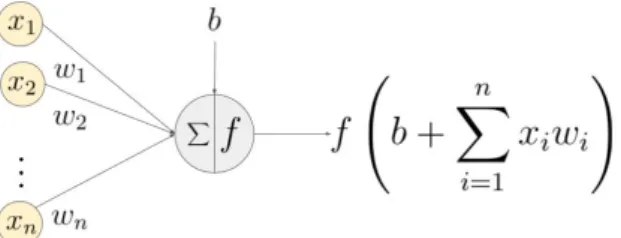
The hidden layer is located in the middle layer of the network and it’s composed of hidden neurons, also known as hidden units. Each of these neurons will receive a weighted sum from the neurons of the previous layer. This operation is followed by the application of an activation function (e.g. ReLu function) to the weighted sum (Fig. 2.3). Using an activation function introduces non-linearity into the output layer, allowing the separation of data that’s not linearly separable.

Once the activation function has been applied, the neurons will output their results to the next layer (i.e. output layer).

Figure 2.3: Application of an activation function f to the weighted sum of the inputs. Extracted from [34].

The output layer is the last layer of the neural network and it’s used to compute the model’s output value (i.e. prediction). Depending on the problem assigned to the model, the output can assume the shape of a regression (e.g. predict the numeric price of a house) or a classification (e.g. predict whether a profile image has good quality or not). This dissertation’s proposed work is a classification type of problem.

(36)

Training a neural network

In order to have a model consistently performing correct predictions, it is necessary to train it first. Using a supervised learning approach, the model is fed with training data from which the correct output for each training sample is already known. For each training sample, the model will compute an output (i.e. forward-pass), which is then compared with the sample’s correct output. A cost function is used to measure the difference between the model predictions and the desired outputs, which reflects how well the model is doing. As previously mentioned, adjusting the weights and biases of the model will result in different predictions, therefore it’s necessary to find out exactly what adjustments need to be made, to lower the cost. To do that, back-propagation [41] is used to compute the model gradients, by repeatedly using the chain rule. Based on the choice of the optimizer (e.g. SGD, Adam [28]), these gradients will be used to update the weights and biases of the model, and consequently lower the cost.

Training a model consists essentially of the repetition of these 4 steps: forward-pass, calculation of the cost, back-propagation, and the update of the parameters. Once the model’s training has been completed, it can be tested on a test dataset to evaluate how well is it capable of making predictions using data not yet seen by the model (i.e. generalization).

Deep neural networks

The way that a deep neural network works is quite similar to the way a shallow neural network does (i.e. the input layer is fed with data that goes through the hidden layers and ends up in the output layer, resulting in a prediction). The difference between the two architectures is the number of hidden layers the data must pass through, as deep architectures consist of two or more hidden layers. Since deep architectures have multiple hidden layers, the input data will also pass through more activation functions. As a consequence of that, the model is able to learn more complex and difficult data representations (e.g. images, video, voice-recognition). Deep architectures have also better performance [23] and gen-eralization [7] compared to shallow architectures.

Another important aspect about deep networks is their ability to automatically

(37)

extract relevant data features [29], without being specifically taught to do so (i.e. end-to-end). Unlike deep neural networks, the traditional computer vision algo-rithms require the features to be manually engineered, which can be very time consuming and expensive.

Although deep architectures perform better than shallow architectures, there are also some less positive aspects to it, such as being much more computationally expensive due to their size (i.e. more hidden layers corresponds to more parame-ters). These models need a lot more data to learn, and they also take a lot longer to train (e.g. weeks).

2.2.1.2 Activation functions

Each neuron in the hidden layers of a network has an activation function assigned to it. The fact that these activation functions are nonlinear functions, allows the model to learn more complex functions and data representations (Fig. 2.4), in order to solve difficult and non-linearly separable problems [22].

Figure 2.4: Representation of linear data (left) and non-linear data (right). Extracted from [40].

The popular activation function’s choice for the hidden layers is usually the rec-tified linear unit (ReLu) f (x) = max(0, x). Among other activation functions like the traditional sigmoid and tanh, ReLu is a safe choice due to the fact that unlike sigmoid and tanh, it rarely suffers from vanishing gradient [33], and it also introduces sparsity to the network [20], which improves the process of analyzing and extracting features from the data.

(38)

2.2.1.3 Regularization

When a neural network model is learning from the training data, there is a possi-bility that the model will start to overfit to the data. This means that the model will perform extremely well on the training data but it’ll have a poor generaliza-tion on new and unseen data. This is a big problem for neural networks since the main goal of training them is to use them to perform tasks on new data.

Regularization is used to prevent the overfitting problem which is very important when training a neural network. A deep neural network is more prone to overfit the data compared to shallow networks, because of the bigger number of parame-ters introduced into the network [46].

A regularization method such as the Dropout [46] is a way to address overfitting the data. Dropout consists of picking random neurons and just drop them from the network during training. This prevents the neurons from adjusting too much to the training data, resulting in a more balanced model that’s able to generalize unseen data.

2.2.2 Convolutional neural networks

A convolutional neural network [30] also known as (CNN) is a type of deep neural network designed to process images as the main input, which proved to be very powerful when used on visual recognition tasks [29, 51, 23, 44] leading to huge advances in the computer vision field and completely outperforming architectures that used feature-based approaches, such as the scale-invariant feature transform (SIFT) [31], and the speeded up robust features (SURF) [6] approach.

2.2.2.1 The layers of a CNN

A CNN is typically composed of three different layer types: a convolutional layer, a pooling layer, and a fully-connected layer.

(39)

Convolutional layer

A convolutional layer [30] (CONV) consists of sliding a collection of learnable filters (or kernels) of a fixed size, over the input data (e.g. profile image) in a sliding window manner. The region of the input covered by a filter is called the receptive field. These filters work like feature detectors where each filter looks for some specific characteristic present in the input data (e.g. edges, curves). For each region of the input data covered by the filter, it’s performed a dot product between the filter’s matrix and the matrix of the region covered, and everything is summed into one value (i.e. convolution operation, Fig. 2.5) followed by the application of a ReLu function. Once the filters slide across the whole input, this will result in a feature map composed of all the convolution operations done to the input data.

Figure 2.5: Example of a convolution operation. Extracted from [54].

Assuming the convolutional layer is the first layer of the CNN, this layer will start looking at low-level features. These low features can be something as simple as edges or curves. Adding a second convolution layer on the output of the first convolutional layer will generate even more complex features and shapes such as circles or squares. Increasing the number of convolutional layers used will continue to increase the complexity of the shapes created, making them so abstract that they end up not being visually interpretable by humans.

Pooling layer

The pooling layers (POOL) are usually used after a convolutional layer, and these layers decrease the feature map’s dimensionality for better computational

(40)

effi-cover the input regions. There are two types of pooling layers, the max, and the average pooling layer. When using the max pooling layer, the covered region will output the max value of that region whereas the average pooling layer will output the average of the values from that region.

Figure 2.6: An example of a max pooling operation. Extracted from [35].

Fully connected layers

The fully-connected layers (FC) are usually attached to the end of the CNN serving as output layers, and they work the same way as the regular feed-forward neural networks described previously.

2.2.2.2 Main CNN architectures

In this section, it’s presented an overview of some CNN architectures that have made important contributions to the use of CNN architectures.

AlexNet

The ImageNet Large Scale Visual Recognition Competition (ILSVRC) [42] is an annual competition where different research teams evaluate their algorithms for object detection and image classification at a large scale.

In 2012, AlexNet [29], a convolutional neural network, won the ILSVRC’12 compe-tition achieving a top-5 error (i.e. 1 of the 5 model’s labeled predictions is correct) of 15.4% while the second best achieved a top-5 error of 26.2%. This moment was one of the biggest game changers in modern computer vision. New convolutional neural networks architectures started to emerge [44,51] and other computer vision techniques started to fall off.

(41)

The AlexNet’s architecture consisted of five convolutional layers and three fully-connected layers, with the purpose of classifying images with 1000 possible classes. Using the ReLu nonlinear activation function and highly optimized GPU imple-mentation, the network was able to train much faster.

AlexNet artificially enlarged its training dataset through data-augmentation tech-niques consisting of image patch extractions, translations, and horizontal reflec-tions, which prevented the model from overfitting the data. In addition to these techniques, Dropout [46] was also used. Since AlexNet’s appearance, new CNN architectures began appearing in later ILSVRC competitions.

VGG

The VGG [44] architecture got the second place on the ILSVRC 2014 competition with a top-5 error of 7.3%, and was known for its uniform and simple network. The important contribution of this paper was the discovery that a CONV layer with a large filter could be replaced with multiple CONV layers with 3 × 3 sized filters. This technique maintains the same receptive field and uses fewer parameters. In addition, this also means that more activation functions are used, resulting in better feature extraction.

The drawback of this architecture is that it can be computationally expensive to train due to its number of parameters.

GoogLeNet

The GoogLeNet [51] is a 22-layered architecture that won the ILSVRC 2014 com-petition with a top-5 error of 6.7%.

The main focus of this network was about creating a deeper model that was more computationally efficient, achieved with the introduction of the inception module used in stacked layers, which resulted in a reduction from 60 million parameters (AlexNet) to just 4 million. Some features of this architecture that contributed to this optimization were the use of average pooling layers as classifiers instead of the traditional fully connected layers, and the fact that each of the inception modules used a 1 × 1 convolution filter for dimensional reduction.

(42)

Residual Networks

The Residual Networks (ResNets) [23] won the first place in the ILSVRC 2015 competition with a top-5 error of 3.57%, using a very deep architecture composed of 152 layers.

This model consists of stacking residual learning blocks (Fig. 2.7). These residual blocks are essentially just two stacked CONV layers with an identity mapping shortcut connection that is added to the output of the second CONV layer. This simple technique allows the building of much deeper neural networks and it also addresses the vanishing/exploding gradient problem, that can occur when training regular deep architectures.

Figure 2.7: A residual block. Extracted from [23].

2.2.2.3 Transfer learning

Transfer learning [57] is a special feature of deep learning that allows transferring a model’s knowledge to perform a specific task and apply that knowledge to another task.

The process of transferring learning consists of using a model previously trained on a big dataset (e.g.ImageNet [42]) and replacing its output layer with a new output layer for the new task. The last step is to train the model, and only the new layer is necessary to be trained. Optionally, it’s possible to train more than just the output layer, but that is only recommended if there’s enough training data available, to avoid overfitting.

Transfer learning works because a pre-trained model was already trained to detect common features (e.g. edges, curves, etc) that exist in every object. The use of transfer learning not only eliminates the need for a large amount of training data

(43)

(i.e. millions of labelled images) to train a deep neural network, but also, it de-creases the time it takes to set up a usable model, since it can take weeks just to train a model from scratch whereas it takes only a couple of epochs using transfer learning.

Given these advantages and the fact that the training data available for the pro-posed work may not be sufficient to train a model from scratch, transfer learning is an approach that will be used in this dissertation.

2.2.3 Deep learning frameworks

As deep learning continues to grow and become more popular, deep learning frame-works also keep being developed. There is a wide range of frameframe-works available, from low-level API frameworks such as TensorFlow [2], developed by Google, to high-level API frameworks such as Keras [11], which is more beginner friendlier, and also the framework that will be used in this dissertation.

The process of creating a CNN model is very easy using a framework such as Keras because only a few lines of code are needed to create and stack layers and train the model. In addition, there are pre-trained models available in the framework that can be imported and used immediately to make classifications, or to modify them as needed (e.g. add/ remove/ freeze layers), in order to set the model ready for transfer-learning.

Another advantage of using a framework is that when a model is being trained, the computation of the model gradients and the update of the parameters are carried out by the framework. This feature saves a lot of time in the model implemen-tation process and also prevents potential bugs that could result from manually coding these calculations for millions of parameters.

Finally, the fact that these frameworks are already programmed to run efficiently on a GPU [11], speeds up the training time exponentially. The GPUs are great at parallel processing, and since training a CNN model consists of large matrix computations, the training process becomes a lot faster using them [53]. :

(44)

(45)

Chapter 3 Implementation

To compare the DNN approach against the traditional computer vision algorithm approach, a set of experiments will be performed (one for each requirement) where the classification results, the complexity of the implementation and the computa-tional time associated to the classification process will be taken into account for both methods. In every experiment, a traditional algorithm is implemented and tuned, and a DNN model is trained to classify the compliance of the experiment’s requirement. Each requirement will be individually classified so that it can be determined which specific requirements are or aren’t compliant with the image. In order to tune and train the traditional algorithms and the DNNs used in the experiments, we define two types of datasets for each experiment: (i) a “compliant dataset” composed by a collection of images that are compliant with the respec-tive requirement; and, (ii) a “non-compliant dataset” composed by a collection of images that fail to comply with that requirement. The strategy used to collect images for each of these datasets and the way they’ll be processed is described also in this chapter. The strategy used to collect images for each of these datasets and the way they’ll be processed is described also in this chapter.

(46)

3.1 Dataset

3.1.1 ISCTE-IUL database

Given the purpose of this dissertation, most of the image data used belongs to the ISCTE-IUL database. This database consists mainly of photos of students and employees, taken at shoulder level, with their faces visible, and facing the camera. For each photo, its original and thumbnail versions (max width/height: 100px) are available, however, a big portion of the photos only have their thumbnail version stored, especially the older ones.

The following table presents the ISCTE-IUL database:

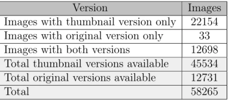
Table 3.1: Initial ISCTE-IUL database.

Version Images Images with thumbnail version only 22154 Images with original version only 33 Images with both versions 23380 Total thumbnail versions available 45534 Total original versions available 23413

Total 68947

After further analysis, it was observed that 10682 images with both original and thumbnail versions available, had their thumbnail versions mistakenly stored as both versions, decreasing even more, the number of images with original versions available. This issue could be verified by checking and comparing the dimensions of both image versions.

After every image had their versions checked and corrected, the following table presents the processed database:

Table 3.2: ISCTE-IUL database after being processed.

Version Images Images with thumbnail version only 22154 Images with original version only 33 Images with both versions 12698 Total thumbnail versions available 45534 Total original versions available 12731

Total 58265

(47)

Only the original version of the images is used on the experiments, as these images are easier to manually label due to their dimensions, and also because the exper-iments will reshape every input images to a dimension of 512 × 512, which could lead to a quality loss if the thumbnail version was used. Of the 12,731 images with original versions available, only a subset of 9,264 images was used and manually labelled due to time constraints and also because this database wasn’t providing enough images to populate most of the non-compliant datasets.

3.1.2 External datasets

Since it’s beneficial performance-wise to provide the DNN models with more rel-evant and similar image data, and because the ISCTE-IUL database does not contain enough image data to create some of the non-compliant datasets, other external datasets are also used.

The following table lists the datasets from which image data will be collected:

Table 3.3: Datasets used on the experiments.

Dataset ISCTE-IUL database AR Face Database [50] Chicago Face Database [32]

Closed Eyes in the Wild Dataset [45] Face Research Lab London Set [14] MR2 dataset [49]

ImageNet [42]

NimStim dataset [52] PUT Face Database [27] Siblings Dataset [55]

Young Adult White Faces [15]

3.1.3 Datasets for the quality requirements

Since each experiment evaluates a different requirement, it’s necessary to create a different dataset according to the quality requirement being evaluated. Given

(48)

and 1 fully-compliant dataset are required. To that end, the process of creating each dataset is described next.

Compliant dataset

The compliant dataset consists of images in conformance with the quality require-ment being evaluated. Each image from this dataset was carefully selected and collected from the datasets previously mentioned.

Blurred dataset

The blurred dataset is created using images collected from the compliant dataset. Using Python’s OpenCV library [9], two types of blurring methods are applied to the images: Gaussian blur and motion blur.

Unnatural skin tone dataset

The unnatural skin tone dataset is created using images collected from the com-pliant dataset. Using Python’s OpenCV library [9], a yellow toned color is applied to the person’s skin pixels, resulting in an unnatural skin tone color.

Too dark/light dataset

The too dark/light dataset is created using images collected from the compliant dataset. Using Python’s OpenCV library [9], each image’s V channel (HSV color space) is adjusted accordingly, in order to obtain lighter/darker images. Increasing the value of the V channel will generate brighter images whereas doing the opposite will generate darker images.

Pixelation dataset

The pixelation dataset is created using images collected from the compliant dataset. Using Python’s OpenCV library [9], each image is scaled down and scaled back to its original size, generating a pixelation effect.

Washed out dataset

The washed out dataset is created using images collected from the compliant dataset. Using Python’s OpenCV library [9], a white overlay with some trans-parency is added on top of the image, creating a washed out effect.

(49)

Eyes closed dataset

The eyes closed dataset is created using a collection of images from the Closed Eyes in the Wild Dataset and some images carefully selected from Google Images.

Red eyes dataset

The red eyes dataset is created using images collected from the compliant dataset. Using Python’s OpenCV library [9], each individual had a transparent red colored overlay added to their eye pupils, creating the red eyes from flash effect.

Dark tinted lenses dataset

The dark tinted lenses dataset is created by carefully selecting images collected from the AR Face Dataset, from Google Images, and images labeled as sunglasses from the ImageNet dataset.

Hats dataset

The hats dataset is created by carefully selecting images from Google Images and images labeled as a hat from the ImageNet dataset.

Mouth closed dataset

The mouth closed dataset is created by collecting images from the ISCTE-IUL database, the AR Face Database, the Face Research Lab London Set and the NimStim dataset, where the individuals have their mouths open.

At the end of each dataset creation process, in order to maintain consistent image dimensions and also due to the fact that the collected images had originally very different resolutions that could affect each experiment’s performance, every image is scaled down to a maximum width or height of 512, while maintaining its original aspect ratio.

(50)

3.2 Experimental setup

3.2.1 Experiment dataset

An experiment dataset is created for each experiment, consisting of a compliant dataset for the compliant class, and a non-compliant dataset for the non-compliant class. The experiment dataset is split randomly into different sets, to train or tune the algorithms according to the approach used:

• Traditional algorithm: 90% train set, 10% test set. • DNN: 80% train set, 10% validation set, 10% test set

It’s not necessary to generate a validation set for the traditional algorithms used, as overfitting the data is only an issue for the DNN approach.

Once the traditional algorithms have been tuned and the DNN training is com-plete, the performance of both methods is measured on the test set using metrics that will be presented further in this section. In order to ensure a fair comparison of the results, the test sets of both methods are exactly the same.

3.2.2 Experimental environment setup

All experiments are conducted in the same environment: a machine equipped with an NVIDIA TITAN Xp GPU, Intel(R) Xeon(R) CPU E5-2660 0 @ 2.20GHz and 32 GB of RAM.

3.2.3 DNN model setup

VGG-16

Due to its popularity, simplicity, and accuracy, the VGG-16 is the architecture of choice for the DNN approach, on every experiment. Using the Keras frame-work [11], the VGG-16 model can be easily imported and optionally loaded with

(51)

the ImageNet weights for transfer-learning. The input size of the model is set to 512 × 512, as it is desired to classify images with similar dimensions, and its last 3 dense layers are swapped with a flatten and dense layer of two units (two classes), using softmax as the activation function.

Two approaches are analyzed in the training of the DNN model: one consists of training the model from scratch, the other consists of training the model using transfer-learning, since the available training data may not be enough to train a model from scratch without causing overfitting issues.

In each experiment, the model is trained 7 different times, once from scratch, and the other six times using transfer-learning while unfreezing a different number of blocks of convolutional layers each time, as it’s shown in the following table:

Table 3.4: DNN model variants.

Variant Weights Layers

trained Parameters 1 Randomly initialized 14 14,976,834 2 ImageNet 1 262,146 3 ImageNet 4 7,341,570 4 ImageNet 7 13,241,346 5 ImageNet 10 14,716,674 6 ImageNet 12 14,938,114 7 ImageNet 14 14,976,834

From these 7 model variants, the one that provides the best classification results on the validation set is to be selected as the model that classifies the test set.

Hyperparameters

Some hyperparameter optimization was also done in each experiment in order to find the appropriate learning rate, optimizer, and batch-size1. This process consisted of training the model for two epochs2 _{with different parameter values}

and selecting the combination of parameters with the best results on the validation set. The optimizers evaluated were the SGD and Adam, the learning-rates values used were [0.0001, 0.00001, 0.00002, 0.00005], and the batch-sizes were [1, 8, 16, 32]. The batch-size could not be further increased due to memory constraints.

(52)

Since the combination of the Adam Optimizer with a learning rate of 0.0001 and a batch size of 32 performed best in the hyperparameters optimization of every experiment, the combination of these parameters was used in all the experiments. The number of epochs used to train the model was set to 100, even though models using transfer-learning do not require as many epochs as training a model from scratch would.

The Keras callbacks functionality was also used while training the models: the EarlyStop callback to stop the model from training if the validation loss stops improving after 10 epochs, the ModelCheckpoint callback to save the model every time the validation loss decreases, and the ReduceLROnPlateau callback to reduce the learning rate by a factor of 0.5 when the validation loss stops improving every 2 epochs, to help the model reach the minimum cost.

Data augmentation

Data augmentation was performed in each experiment, using the Keras built-in image augmentation functionality. The augmentation techniques used for each experiment were carefully selected, as some of the techniques could negatively affect some datasets and thus degrade the model’s performance. An example of image augmentation misuse would be, applying brightness modifications to the “too dark/light” dataset.

Imbalanced data

Some of the experiment datasets suffered from imbalanced data issues (i.e. size discrepancies between the compliant and non-compliant classes) which could lead to misleading results, therefore, class weight adjustments are performed in each experiment as needed.

The weight adjustments consist of changing the weight of the class from the smaller dataset, to the magnitude of the larger dataset compared to the smaller dataset.

(53)

3.2.4 Metrics

In each experiment, the two approaches’ classification results are compared using the metrics Precision, Recall, and the F1-Score on both classes (using Python’s Scikit-learn library [39]), as well as the computational time associated. To mea-sure a method’s computational time, the test set is classified 10 times, from which the samples with the shortest and longest duration are removed, and an average of the remaining samples is taken to obtain the computational time. This ap-proach is used in order to minimize certain factors associated with setting up the scripts which could affect the computational time of each method (e.g. memory allocation to run the scripts), and thus obtain a value that’s closer to the actual computational time.

3.3 Experiments

In this section, it’ll be performed an experiment for each of the 10 quality re-quirements, where both DNN and traditional algorithms approaches are evaluated regarding the metrics previously mentioned.

3.3.1 Blurred

The following table presents the class composition of this experiment’s dataset:

Table 3.5: Blurred experiment dataset.

Number of images Compliant 6088

Non-Compliant 18259

Traditional algorithm

This algorithm was implemented based on the approach proposed in [38], as de-scribed in section 2.1.1, using the Laplacian and variance function from Python’s OpenCV library [9]. The algorithm was tuned on the training set, which

(54)

con-the best classification results. After furcon-ther threshold tuning, it was determined that images with a Laplacian variance above 45 will be considered compliant.

Deep neural network

Due to the presence of class imbalance issues on this dataset, the following class weights were used:

Table 3.6: Adjusted class weights of the blurred experiment dataset.

Class weights Compliant 3.0 Non-Compliant 1.0

The following data augmentation techniques were used: horizontal flip, rotation range (10◦), conversion to grayscale and brightness adjustment.

The training of the 7 model variants is performed and the final model is selected based on the validation set results. In this experiment, the variant using transfer-learning and trained with 14 layers performed the best (TableA.1).

3.3.2 Unnatural skin tone

Table 3.7: Unnatural skin tone experiment dataset.

Non-Compliant 2057

This algorithm was implemented based on the method proposed in [17], as de-scribed in section 2.1.1. The face region is extracted using the OpenCV cascade and then converted into the YCrCb color space where a color threshold [5] (133 < Cr < 173 and 77 < Cb < 127) is sequentially applied. Finally, the percentage of natural skin within the region is calculated.

The algorithm was tuned on the training set to find the threshold that will define the image as compliant or non-compliant. After further threshold tuning, it was determined that images with natural skin above 60% are considered compliant.

(55)

Deep neural network

Table 3.8: Adjusted class weights of the unnatural skin tone experiment dataset.

The following data augmentation techniques were used: horizontal flip, zoom range (0.05) and rotation range (10◦).

The training of the 7 model variants is performed and the final model is selected based on the validation set results. In this experiment, the variant using transfer-learning and trained with 7 layers performed the best (Table A.2).

3.3.3 Too dark/light

Table 3.9: Too dark/light experiment dataset.

Non-Compliant 11477

The algorithm used in this experiment was implemented based on the method used in [17], as described in section 2.1.1. Using the OpenCV library [9] for Python, the image was converted to grayscale and its color histogram was generated to calculate the compliance score.

While the author’s method outputs an image’s compliance score from [0-100], this algorithm evaluates the images as compliant or not-compliant based on a threshold value that must be tuned. After further threshold tuning, it was determined that images with a score above 60 will be considered compliant.

(56)

Deep neural network

Table 3.10: Adjusted class weights of the too dark/light experiment dataset.

3.3.4 Washed out

Table 3.11: Washed out experiment dataset.

Non-Compliant 6131

The algorithm used in this experiment was implemented based on the method used in [17], as described in section2.1.1. Using the OpenCV library [9] for Python, the image was converted to grayscale and the histogram used to calculate the image compliance score is generated.

While the author’s method outputs the images’ compliance score from [0-100], this algorithm evaluates the images as compliant or not-compliant based on a threshold value that must be tuned. After further threshold tuning, it was determined that images with a score above 70 will be considered compliant.

(57)

Deep neural network

As both classes in this dataset are balanced, no class weight adjustments have been made.

The following data augmentation techniques were used: horizontal flip, zoom range (0.05) and rotation range (10). The training of the 7 model variants is performed and the final model is selected based on the validation set results. In this experi-ment, the variant using transfer-learning and trained with 14 layers performed the best (Table A.4).

3.3.5 Pixelation

Table 3.12: Pixelation experiment dataset.

Non-Compliant 3351

The algorithm used in this experiment was implemented based on the approach proposed in [36], as described in section 2.1.1. Using Python’s OpenCV library [9], the cascade function was used to find the face region which was then converted to grayscale. The Canny edge detector followed by the Hough Transform function was used to detect lines.

While the author’s method outputs the images’ compliance score from [0-100], this algorithm evaluates the images as compliant or not-compliant based on a threshold value that must be tuned. After further threshold tuning, it was determined that images with a score above 50 will be considered compliant.

Deep neural network

As both classes in this dataset are balanced, no class weight adjustments have been made.

(58)

con-final model is selected based on the validation set results. In this experiment, the variant using transfer-learning and trained with 4 layers performed the best (Table A.5).

3.3.6 Eyes closed

Table 3.13: Eyes closed experiment dataset.

Non-Compliant 1798

The algorithm used in this experiment was implemented using the Haar feature-based cascade classifier approach [56], as described in section2.1.1. Using Python’s OpenCV library [9], the cascade function is used to find the face and the eyes regions. The face and the eyes cascades are provided in the library.

The image is considered compliant if the person’s face and both eyes are detected.

Deep neural network

Table 3.14: Adjusted class weights of the eyes closed experiment dataset.

The following data augmentation techniques were used: horizontal flip, zoom range (0.05), rotation range (10◦), conversion to grayscale and brightness adjustment. The training of the 7 model variants is performed and the final model is selected based on the validation set results. In this experiment, the variant using transfer-learning and trained with 14 layers performed the best (TableA.6).

(59)

3.3.7 Red eyes

Table 3.15: Red eyes experiment dataset

Non-Compliant 830

The algorithm used in this experiment was implemented based on the approach proposed in [17], as described in section2.1.1. Using Python’s OpenCV library [9], the cascade function is used to find each eye region from which the red-eye pixels are identified based on a color threshold [58]. This algorithm uses the percentage of red pixels within the eye regions to classify the image’s compliance. After further tuning the threshold value, it was determined that images with a presence of red pixels below 20% will be considered compliant.

Deep neural network

Table 3.16: Adjusted class weights of the red eyes experiment dataset.

(60)

Table 3.17: Dark tinted lenses experiment dataset

Non-Compliant 1833

This algorithm was implemented using the histogram intersection approach [50], as described in section 2.1.1, which is implemented in a Python library called Deepgaze [37]. The algorithm starts by extracting the eyes region from the image as an input image, which is used to compute the histogram intersection with previously stored images of extracted eye regions of people who are and who aren’t wearing sunglasses.

If the stored image that is the most similar to the input image belongs to a person not wearing dark tinted lenses, the image is considered compliant.

Deep neural network

Table 3.18: Adjusted class weights of the dark tinted lenses experiment dataset.

The following data augmentation techniques were used: horizontal flip, zoom range (0.05), rotation range (10◦), conversion to grayscale and brightness adjustment. The training of the 7 model variants is performed and the final model is selected based on the validation set results. In this experiment, the variant using transfer-learning and trained with 4 layers performed the best (Table A.8).

Deep neural networks for image quality: a comparison study for identification photos

University Institute of Lisbon

Department of Information Science and Technology