SOURCES OF OUTPUT GROWTH IN THE PORTUGUESE ECONOMY (1959·1974) ()

Estudos de Economia, val. II, n.' 3, Abr.-Jun., 1982

SOURCES OF OUTPUT GROWTH IN THE PORTUGUESE

ECONOMY (1959·1974)

(*)

Joao Cravinho

(* *)

1 - Introduction

This paper reports the results of an input-output analysis of the sources of growth in the Portuguese economy in 1959-1974, using the Torii-Fukasaku methodology. Other papers will report research on the same topic using alternative methodologies and extending the problems investigated into the value added and employment areas.

The plan of the paper is as follows: section 2 registers the Torii-Fukasaku method of measurement; section 3 provides a simple over-view of results to the economy as a whole; section 4 details findings for each of the three subperiods 1959-1964, 1964-1970 and 1970-197 4; section 5 comments the results of a decomposition of final demand changes in three categories: private consumption, Government consumption and investment; section 6 closes the report with a set of conclusions.

2 - Methodology

The methodology used in this study has been developped by Torii and Fukasaku (1).

Let it be:

t:.X- Incremental output vector;

A -Technical coefficients matrix;

M

M,- Final import vector;

F d - Domestic final demand vector;

1\-Symbol of diagonal matrix.

(*) Special thanks are due to Manuela Santa Maria, under whose directions the 1-0 tables have been prepared, and to T. Teixeira, who programmed and run the computations.

(**) GEBEl and IDS, Sussex.

(1)

(2)

(3)

From:

X

=

+

+

1\

Mm

=

1\

M,

=

X= [1-(/-Mm)Ar[(l-0,) Fd

+

=

where

B

(4) 11X = X1- X0

::::: 8 1 G1- 8° G0 = 81 ~G

+

Denoting by B * and G * the following matrix and vector:

[ 1\

]·1

(5) B *

=

1\

(6) G*=[(I-M?)Fd1 _+E1

]

and writing:

(7)

(8)

118 = 81

- 8° = (81- B *)

+

t.

- G *)

+ (

we see that 11 X can be decomposed as follows: 1\

fiX= 81

( / -M,0) (Fd1- Fd0)

+

£0)

1\ 1\

+

1\

+

- 8 *)

[(1-

+

£0]

1\

+

[(1-

+

£0)]

Each of these terms measures the effects of a particular source of growth:

a) The first term, the effects of changes in domestic final demand;

b) The second term, the effects of changes in exports;

c) The third term, the effects of changes in final import coefficients;

d) The fourth term, the effects of changes in intermediate import coefficients;

e) The fifth term, the effects of changes in technical coefficients.

Firstly, we can find in the literature other approaches. Secondly, even if we only c.onsider the approach expressed in (4), we can depart from the Torii-Fukasaku solution and find a different way of decomposing ~X. These issues will be dealt with in other papers. At this stage it suffices to note that we may rearrange the second member of (4) as follows:

(9) 81 _.!lG

₊

₌

+

+

=

₊

In the first member, the second term, ~ 8G0

, computes the effect of

changing technology from 81 _{to 8° holding final demand constant at the G}0

level, while the first term, 81 _{~G. computes the effect of changing final}

demand from G1 _{to G}0 _{holding technology constant at the new position 81.} Comparing with the second member, we can see that the first term, 8° ~G. takes the effect of final demand change ~ G assuming that technology is held at the 8° position and, then, computes the effect of changing technology to 81 _{assuming final demand at the G}1 _level.

Of course, the two solutions will lead to different results. In this paper I shall stick to the decomposition expressed in (4).

3 -Output changes in 1959·1974: an over-view

The decade and a half that runs from 1959 to 197 4 has seen remarkable changes in the Portuguese output structure. For 1959, 1964, 1970 and 197 4, for each of these years, we have an 1-0 table in current prices, as compatible as possible, prepared by Manuela Santa Maria and collaborators (2

).

Applying the preceding methodology we get the following broad picture of the sources of changes in output growth.

TABLE I

Sources of total output growth in the economy (1959-1974)

Final demand ... . Exports ... . Import substitution ... .

Final imports ... .

Intermediate imports ... .

1959·1964

85.1 17.2 0.9

2.0 1.1

1964-1970

70.8 20.8 0.7

0.8 1.5

Percentage

1970·1974

94.2 22.5 11.3

6.6 4.7

Technical coefficients

Total ... .

· · · ·1

10~-

_I

_10~·

_{I -}

_10~.4

By far, the most important source accounting for output growth in the economy in the period 1959-197 4 was final demand. Its share in 1970-197 4 attained 94 %. In the two previous subperiods, it has been 71 % in

1964-1970 and 85% in 1959-1964. Exports were the next important source, rising regularly from 17% in 1959-1964 to 22.5% in 1974, a clear signal of the growing openness of the Portuguese economy.

Another relevant signal pointing in the same direction can be read in the import substitution results. Overall, import substitution has been a very secondary factor, although positive, in 1959-1964 and 1964-1970. In each of these subperiods total relative import substitution effects have represented less than 1 % of output growth. Decomposing further import substitution, in final and intermediate uses, we can see that rather small contributions, around 1 % or 2 %, with different signs in different subperiods, were involved. This situation has dramatically changed in the early 70's. Then, total import substitution played a non-negligible role, and a negative one, for that matter, representing - 11.3 % of total growth. Final import substitution alone accounted for - 6.6 %, the remaining - 4. 7 % being earmarked to changes in intermediate import coefficients.

4 - Patterns of changes in the various subperiods

The analysis of the different subperiods will take in turn effects centered on final demand, exports, import substitution and technical change, as measured by change in the input-output coefficients. For each of these sources of output changes two types of developments will be examined. First, the relative contribution of the effect to sectoral output growth, noting the most striking features at sectoral level. Second, the sectoral _ shares relative to the total for the economy shown by the particular effect under study, noting again the most important sectoral features under this approach.

4.1 - 1959-1964

Table 11 confirms the overwhelming importance of final demand effects for all branches in this subperiod. Pulp and paper is the single branch where final demand effects are exceeded by some other type of changes, exports, in the case.

TABLE II

Sources of output growth (1959-1964) (*)

Sectors FD

1 Agriculture and fishing ... 108

2 Mining ... 317

3 Food, beverages and tobacco ... 90

4 Textiles ... 70

5 Apparel, shoe and leather ... 69

6 Wood, cork and furniture ... 80

7 Pulp and paper ... 34

8 Chemicals ... ... 67

9 Petroleum and coal ... 107

10 Non-metalic mineral products . . . 99

11 Basic metallurgy ... 63

12 Metalworking . . . . . . ... ' 68

13 Shipbuilding and repair . ... 746

14 Miscellaneous manufacturing ... 259

15 Electricity, water and gaz ... 76

16 Construction ... 98

17 Trade ... ,. 67

18 Transportation and communications 58 19 Other services ... 104

20 Government ... 100

(") Apart from rounding errors, FD + E + M + A = 100 %.

FD - Final demand effects.

E-Exports.

M-Total import substitution effects (M = MF + MM). MF-Final import substitution effects.

MM - Intermediate import substitution effects.

A -Technical coefficients.

E M

35 - 19

21 -429

- 3 4

46 - 5

29 4

39 1

38 23

37 - 3

- 8 18

17 8

20 33

11 39

-66 -204

41 - 39

11 0

0 0

11 - 12

35 1

0 0

0 0

Percentage

MF MM A

- 8 - 10 - 24

-483 54 0

- 1 5 9

0 - 5 - 11

3 1 - 2

0 0 - 20

22 1 3

- 7 4 - 1

17 - 1 - 14

8 0 - 23

11 22 - 17

49 - 9 - 18

3 -207 -376

- 35 - _{3 -161}

0 0 11

0 0 1

1 0 22

0 - 12 19

1 0 5

0 0 0

It should also be mentioned a second group of industries which benefited from final ·demand impulses to the point of recording higher than average relative levels. This is the case of food, beverages and tobacco, non-metallic mineral products and construction.

The above mentioned pattern matches closely what one could expect in a country approaching the semi-industrialized stage after a decade and a half of an industrialization spurt, in the beginning very much centered in the domestic market, followed by a selective export drive.

Although the role of exports was still modest at that time, for a few sectors it was already a growth factor of some importance. The industries that benefited most, predictably enough, were natural resources based or light labour intensive manufacturing, with two exceptions. Thus, mining, agriculture and fishing, textiles, wood, cork and furniture, apparel, pulp and paper and miscellaneous manufacturing were naturally found among the front runners. Chemicals and transportation and communications were also included in that same group. According to table 11, in all those sectors exports accouted for more than 1{3 of output growth.

In two cases, petroleum and food and beverages and tobacco, the export .effect has been mildly negative. In a single case, shipbuilding, it has been strongly negative.

TABLE Ill

Sectoral shares in output growth effects (1959-1964) (*) _Percentage

Sectors FD E M MF MM A

1 Agriculture and fishing ... 10.7 17.2 -188.9 35.5 80.8 64.3

2 Mining ... 1.4 4.6 -185.5 - 90.1 -17.7 0.0

3 Food, beverages and tobacco ... 14.8 - 2.6 62.1 - 11.1 -66.6 - 42.1

4 Textiles ... 6.1 19.8 - 45.5

-

5 Apparel, shoe and leather ... 4.1 8.5 25.4 8.2 - 4.8 3.1

6 Wood, cork and furniture ... 2.5 6.0

-

7 Pulp and paper ... 0.8 4.3 52.3 21.6 - 1.7 - 2.3

8 Chemicals ... 3.4 9.4 - 16.6 - 15.8 -15.2 1.7

9 Petroleum and coal ... - 0.8 0.3 - 12.3 - 5.8 - 0.9 - 3.1

10 Non-metalic mineral products ... 2.8 2.4 21.3 10.3 1.8 17.6

11 Basic metallurgy ... 2.2 3.6 117.1 17.3 -58.4 16.4

12 Metalworking ... 6.1 5.0 350.9 188.6 65.4 44.4

13 Shipbuilding and repair ... 0.6 - 0.3 - 17.5 0.1 13.4 8.7

14 Miscellaneous manufacturing ... 1.1 0.9 1.6 - 6.3 1.2 18.1

15 Electricity, water and gaz ... 2.0 1.5 0.0 0.4 - 0.7 - 8.1

16 Construction ... 12.2 0.2 10.9 0.2 0.3 - 5.0

17 Trade ... 13.0 10.6 - 69.6 12.2 13.3 -114.5

18 Transportation and communications 3.4 10.1 8.8 0.4 53.6 - 30.3

19 Other serl(ices ... 8.9 0.3 0.0 4.4 1.1 12.8

20 Government ... 7.1 0.0 0.0 0.0 0.0 0.0

(•) Column elements do not sum up to 100% due to the existence of a residual sector imposed by the need to make the 1959 and 1964 tables as compatible as possible with those for 1970 and 197 4.

FD-Final demand effects.

E-Exports.

Regarding the main contributors to total export growth, table 111 points to two sectors far apart from the others, that is, textiles (19.8%) and agriculture ans fishing (17.2 %). This is in perfect agreement with the Portuguese entrepreneurs reaction to the new prospects opened up by the EFTA agreement.

We turn now to import substitution effects.

Over the whole economy, total import substitution effects have been negligible. However, at sectoral level one cannot help to be impressed by significant movements in opposite directions and, thus, offsetting each other.

Concerning relative contributions of IS effects to sectoral growth, in a few cases there has been a pronounced positive effect. This happened in metalworking (39.2 %), in basic metallurgy (33.4 %) in pulp and paper (23.3 %) and in petroleum and coal (15.6 %).

In general terms, these developments are easily explained by the industrialization policy followed in the 50's and early 60's, particularly by means of State support to capital intensive IS substitution projects. The first and second Pianos de Fomento are there to prove the assertion, with the inclusion of investments in oil refinery, stteel and pulp facilities. At the same time, State coordinated linkages with the development of heavy metalworking fabrication and support to smaller firms in the very incipient metalworking industry explain the importance of the IS effect in metalworking.

Next to this first lot, we also find positive import substitution in non-metalic mineral products (7.7 %), though at a much lower level.

In general, for most sectors IS effects in final demand have been higher than in intermediate demand, the obvious exception being basic metallurgy.

Negative IS has been most relevant in agriculture and fishing ( - 19.3 %), in mining (- 429.4 %), shipbuilding and repair(- 203.9 %). The first sector has almost always been at the root of a persistent foreign exchange drag. Overall, at the economy level, the interesting point is that in the early 60's the import substitution phase had already passed its peak and a clear reversal in trends was already visible in important sectors.

Reading table 111, it is clear that a very high share of IS effects in final use occurred in metalworking (188.6% ), while the significant negative shares in the same effect are to be atributed to mining (- 90.1 %) and agriculture and fishing (- 35.5% ). Relative to intermediate IS, agriculture (80.8% ), metalworking (65.4%) and trade (33.6%) are the main positive contributors and food, beverages and tobacco (- 66.6 %) and basic metallurgy (- 58.4%) are their counterparts on the negative side. However, these developments are of little significance, given the negligible size of total IS effects.

Changes in technical coeficients had very negative effects in shipbuilding and repair (- 376.1 %) and miscellaneous (- 161.2%) and

significantly negative (around - 20 %) in several important branches. Positive changes of the last order of magnitude occurred in services and infra-structures. Of course, we must appraise in favourable terms technical changes which save inputs and, thus, lead to a decrease in intermediate demand.

Considering the relative levels of the different effects in mining, we must remember that the absolute output increment is fairly small and results from movements in opposed directions, according to the type of effect. This explains their high percentual representation relative to total effect. This fact has to be keptin mind along this paper.

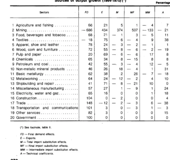
4.2-1964-1970

In the second half of the 60's, final demand impulses for agriculture and manufacturing outputs lost part of their relative strength. However, they have consolidated their position in construction and services sectors, as can be seen in table IV.

TABLE IV

Sources of output growth (1964-1970) (*)

Sectors

1 Agriculture and fishing ... 2 Mining ... 3 Food, beverages and tobacco ... 4 Textiles ... 5 Apparel, shoe and leather ... 6 Wood, cork and furniture ... 7 Pulp and paper ... 8 Chemicals ... 9 Petroleum and coal ... 10 Non-metalic mineral products ... 11 Basic metallurgy ... 12 Metalworking ... 13 Shipbuilding and repair ... 14 Miscellaneous manufacturing ... 15 Electricity, water and gaz ... 16 Construction ... 17 Trade ... 18 Transportation and communications 19 Other services ... 20 Government ...

(") See footnote. table II.

FD-Final demand effects. E-Exports.

M -Total import substitution effects. MF-Final import substitution effects. MM-Intermediate import substitution effects. A - Technical coefficients.

FD 66 -686 68 - 18 78 72 20 65 42 46 62 64 41 57 65 104 148 101 82 100

E M

21 5

434 374

21 - 1

75 6

24 - 3

55 - 8

69 - 6

34 8

55 -. 3

26 18

38 2

24 - 12

71 - 8

27 1

16 0

0 - 2

-12 - 2

3 0

3 0

0 0

Percentage

MF MM A

1 - 4 7

507 -133 - 21

3 - 5 11

- 4 9 38

- 2 - 1 1

- 6 - 2 - 19

- 6 17 8

- 15 8 8

- 4 12 - 5

- 4 1 31

26 - 7 - 18

- 2 4 10

- 21 10 0

- 9 1 24

0 1 18

0 0 4

- 3 6 - 38

- 3 1 - ₃

0 0 15

In manufacturing, final demand relative effects were stronger than the average in the economy in apparel, shoe. and leather (78.4 %) and wood, cork and furniture. Comparing with the previous subperiod, this move, in conjunction with the strength observed in construction and services, could be taken as evidence of consumer demand shifts in agreement with rising incomes.

From the vantage point of sectoral contributions to total final demand effects, services (21.8% ), outdistances any other sector, followed by metal-working (1 0.8% ), agriculture and fishing (1 0.1 % ), food, beverages and to-bacco (9.6 %) and apparel, shoe and leather (9.2 %). By comparison with the 1959-1964 period, trade and construction dropped out of the small group of sectors accouting for most of the final demand effects.

The late 60's confirmed the widening role played by foreign demand for ligth or resource based manufactures in the Portuguese industrialization.

TABLE V

Sectoral shares in output growth effects (1964-1970) (*)

Sectors

1 Agriculture and fishing ... 2 Mining ... 3 Food, beverages and tobacco ... 4 Textiles ... 5 Apparel, shoe and leather ... 6 Wood, cork and furniture ... 7 Pulp and paper_ ... 8 Chemicals ... 9 Petroleum and coal ... 10 Non-metalic mineral products ... 11 Basic metallurgy ... 12 Metalworking ... 13 Shipbuilding and repair ... 14 Miscellaneous manufacturing ... 15 Eleetricity, water and gaz ... 16 Construction ... 17 Trade ... 18 Transportation and communications 19 Other services ... 20 Government ...

(") See note, table Ill.

FD - Final demand effects.

E-Exports.

M-Total import substitution effects. MF-Final import substitution effects.

-MM-Intermediate import substitution effects. A - Technical coefficients.

FD 10.1 1.8 9.6 - 1.0 9.2 1.4 0.6 4.7 0.7 1.1 1.2 10.8 0.6 2.3 2.3 7.7 6.8 8.0 21.8 4.1

E M MF

11.0 72.9 - 6.2

4.0 100.3 -123.8

10.2 - 15.5 - 45.0

14.7 34.7 19.1

9.4 - 33.2 22.9

3.5 - 15.0 10.3

6.5 - 16.6 14.7

8.4 - 54.1 99.3

3.1 13.3 - 6.9

2.1 - 7.9 9.4

2.6 36.6 - 46.4

14.0 30.1 36.7

3.3 - 16.1 27.2

3.7 - 30.9 33.5

2.0 2.7 0.1

0.1 0.2 0.1

- 2.0 11.0 14.7

1.0 - 12.0 20.5

2.4 - 0.3 5.8

0.0 0.0 0.0

'

- - - -

-Percentage

MM A

31.5 10.2

- 1.7 - 0.5

-31.0 14.4

26.5 20.1

- 3.9 0.9

- 1.7 - 3.3

- 0.2 4.3

26.2 5.1

9.9 - 0.7

1.2 6.9

- 6.8 3.4

33.5 16.1

6.6 0.0

2.8 9.0

1.3 - 5.7

0.2 2.9

12.9 - 1.6

5.1 - 2.1

2.9 36.1

The outstanding export led drive in this period has. been centered on textiles; while in 1959-1964 exports represented the source of 46% of sec-toral output growth, in 1964-1970 they represented 74%.

This upward trend ·also characterized other manufacturing sectors, which could take advantage of natural resources or labour availabilities. Food, beverages and tobacco, from - 3% to 21 %, wood, cork and furni-ture, from 39% to 55%, and pulp and paper, from 38% to 69%, based their success on primary resources. The change in shipbuilding and repair, from - 66% to 71 %, is explained by the start up of the huge LISNAVE ship repair facilities, manned by an adaptable and low paid, by international standards, labour force. The same advantage explains the wider role of for-eign markets in metalworking output growth, which more than duplicated its relative contribuition, from 11 % to 24%.

In· three other sectors the need to gain economies of scale created temporary excess capacity which has been allocated to some extent to foreign markets. This happened in petroleum, chemicals and basic metallurgy. Ex-port relative shares in sectoral growth have gone in the first case from -8% to 55%; in the second case, from 38% to 55%, and in the third case, from 21 % to 38%. Now, concerning the weight of each sector in to-tal export growth, the outstanding position goes to textiles (14.7 %) and met-alworking (14.0 %), followed by agriculture and fishing (11.0 %), food, bev-erages and tobacco (1 0.2%) and apparel, shoe and leather (9.4% ).

Negative import substitumintion in final uses is the pervasive feature of the 1964-1970 evolution. Apart from the very hight percentual change in min-ing, significant positive import substitution in final use occurred only in the case of metallurgical products.

On intermediate uses, mild positive import substitution effects in sev-eral sectors reflect the development of basic industries initiated in the mid 50's and furthered in the 60's.

Changes in technical coefficients have been an important positive source for some sectors: textiles (38 %), non-metalic mineral products (31 %) and miscellaneous (24%) are the clearest cases. On the other hand, the same source has shown to be noticeably negative in mining (- 21 %), wood, cork and furniture.(- 19 %), basic metallurgy (- 18 %) and in trade (- 38 %). The first set of results needs to be researched further.

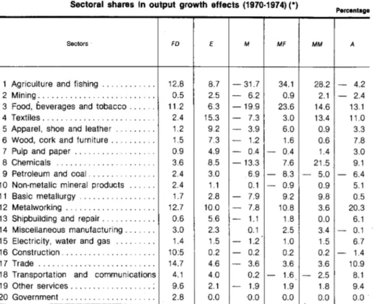
4.3 - 1970-1974

In the early 70's domestic final demand reinforced its relative strength as a source of growth for every sector but for the export nucleous built around textiles, apparel and wood and cork activities.

sec-toral output growth. With the exception of petroleum, which has benefited from a broad, diversified support for output growth, the last group of sec-tors turned to export led growth.

The highest contributions to total final demand effects were found in trade (14.7 %), agriculture and fishing (12.8 %), metalworking (12.7 %), food, beverages and tobacco (11.2 %) and construction (1 0.5% ).

As already mentioned, export led growth prevailed in a few sectors which had already started their foreign demand orientation in earlier periods.

'

The 1970-197 4 developments only extended their commitment to such growth path. Exports were specially important as a source of growth in tex-tiles (81 %), apparel, shoe and leather (80 %), wood, cork and furniture (65 %), pulp and paper (64 %) and shipbuilding and repair (93 %). In chemi-cals (59%) and in basic metallurgy (54%), excess capacity due to econo-mies of scale help to explain export results.

TABLE VI

Sources of output growth (1970·1974) (*)

Sectors FD

1 Agriculture and fishing ... 113

2 Mining ... 104

3 Food, beverages and tobacco ... 117

4 Textiles ... 52

5 Apparel, shoe and leather ... 44

6 Wood, cork and furniture ... 57

7 Pulp and paper ... 48

8 Chemicals ... 103

9 Petroleum and coal ... 55

10 Non-metalic mineral products ... 101

1.1 Basic metallurgy ... 140

12 Metalworking ... ' ... 98

13 Shipbuilding and repair ... 40

14 Miscellaneous manufacturing ... 84

15 Electricity, water and gas ... 114

16 Construction ... 99

17 Trade ... 100

18 Transportation and communications 85 19 Other services ... 103

20 Government ... 100

(") Apart from rounding errors. FD + E + M + A = 100 %.

FD-Final demand effects. E-Exports.

M-Total import substitution effects (M = MF + MM). MF-Final import substitution effects.

MM-Intermediate import substitution effects. A -Technical coefficients.

E M

18 - 34

121 -153

16 - 25

81

-

80 - 17

65 - 5

64

-

59 - 46

17 19

11

-

54 - 92

18 - 7

93 - 9

16 0

29 - 11

0 0

7 - 3

20 5

5 - 2

0 0

Percentage

MF MM A

21 12 2

-131 - 22 28

-

- 5 - 15 - 14

- 15 - '1 - 7

- 4 - 1 - 17

1 - 3 - 9

-

13 6 8

3 2

-

- 53 - 39 - 2

- 6 - 4 - 9

- 9 0 - 25

5 - 5 0

- 5 - 6 - 32

0 0 1

- 2 - 1

-

2 3

-

- 1 - 1 - 6

0 0 0

TABLE VII

Sectoral shares In output growth effects (1970·1974) (*)

Sectors

1 Agriculture and fishing ...

2 Mining ...

3 Food, beverages and tobacco ...

4 Textiles ...

5 Apparel, shoe and leather ...

6 Wood, cork and furniture ...

7 Pulp and paper ...

8 Chemicals ...

9 Petroleum and coal ...

10 Non-metalic mineral products ...

11 Basic metallurgy ...

12 Metalworking ...

13 Shipbuilding and repair ...

14 Miscellaneous manufacturing ...

15 Electricity, water and gas ...

16 Construction ...

17 Trade ...

18 Transportation and communications

19 Other services ...

20 Government ...

(*) See note, table Ill. FD - Final demand effects. E-Exports.

M-Total import substitution effects. MF-Final import substitution effects.

MM - lnterm,ediate import substitution effects. A - Technical coefficients.

FD E

12.8 8.7

0.5 2.5

11.2 6.3

2.4 15.3

1.2 9.2

1.5 7.3

0.9 4.9

3.6 8.5

2.4 3.0

2.4 1.1

1.7 2.8

12.7 10.0

0.6 5.6

3.0 2.3

1.4 1.5

10:5 0.2

14.7 4.6

4.1 4.0

9.6 2.1

2.8 0.0

M MF

-31.7 34.1

- 6.2 0.9

-19.9 23.6

- 7.3 3.0

- 3.9 6.0

- 1.2 1.6 - 0.4 - 0.4

-13.3 7.6

6.9 - 8.3 0.1 - 0.9

- 7.9 9.2

- 7.8 10.8

- 1.1 1.8

0.1 2.5

- 1.2 1.0

- 0.2 0.2

- 3.6 3.6

0.2 - 1.6

- 1.9 1.9 ·0.0 0.0

Percentage

MM A

28.2 - 4.2 2.1 - 2.4 14.6 13.1

13.4 11.0

0.9 3.3

0.6 7.8

1.4 3.0

21.5 9.1

- 5.0 - 6.4

0.9 5.1

9.8 0.5

3.6 20.3

0.0 6.1

3.4 - 0.1

1.5 6.7

0.2 - 1.4 3.6 10.9

- 2.5 8.1

1.8 9.4

0.0 0.0

A sizeable proportion of total export growth has been due to textiles (15.3%), apparel, shoe apd leather (9.2%) and metalworking (10.0%); the latter in spite of its relative orientation in favour of the domestic market.

Regarding intermediate uses, the almost universal result has been neg-ative import substitution. The most serious relneg-ative development concerns basic metallurgy (- 39 %) and chemicals (- 31 %) but textiles (- 12 %) and agriculture (- 15%) should also be mentioned.

Changes in technical coefficents have also been a negative source of growth for the 16 out of 20 sectors. This is in line with what we might ex-pect.

5 - .-nvate consumption, Government consumption and investment expenditures as sources of growth

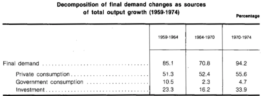
Final demand changes have been the dominant source of growth in any of the subperiods. As already stated (til.ble 1), the record shows that they provided for 85% of total growth in 1959-1964, 71% in 1964-1970, and 94% in 1970-1974. Now, we are going to examine the decomposition of final demand changes into three components, that is, private consumption, Government consumption and investment changes.

Table VIII shows the impact of each of these sources in total output growth in the economy from 1959-1974.

TABLE VIII

Decomposition of final demand changes as sources of total output growth (1959-1974)

1959·1964 1964·1970

Final demand ... ... 85.1 70.8

Private consumption ... 51.3 52.4

Government consumption .. ... 10.5 2.3

Investment ... 23.3 16.2

Percentage

1970·1974

94.2

55.6 4.7 33.9

The results obtained provide valuable insights into the consequences of economic policies followed in the 60's and early 70's.

Firstly, to accomodate the resources mobilization for military use, following the outbreak of guerilla warfare in the three African colonies -Angola, Mozambique and Guine - . Government consumption and investment growth rates have been severely reduced in. the second half of the 60's. This explains the drop of final demand changes share in total output growth from 85% in 1959-1964 to 71% in 1964-1970.

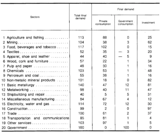
TABLE IX

Private consumption, Government consumption and investment effects (1959-1964)

Sectors

1 Agriculture and fishing ... . 2 Mining ... . 3 Food, beverages and tobacco ... . 4 Textiles ... . 5 Apparel, shoe and leather ... . 6 Wood, cork and furniture ... . 7 Pulp and paper ... . 8 Chemicals ... . 9 Petroleum and coal ... . 10 Non-metalic mineral products ... . 11 Basic metallurgy ... . 12 Metalworking ... . 13 Shipbuilding and repair ... . 14 Miscellaneous manufacturing ... . 15 Electricity, water and gas ... . 16 Construction ... . 17 Trade ... . 18 Transportation and communications 19 Other services ... . 20 Government ... .

Total final demand 113 104 117 52 44 57 48 103 55 101 140 98 40 84 114 99 100 85 103 100 Private consumption 88 38 102 35 40 22 30 53 38 18 47 40 5 67 72 2 61 81 97 0

Final demand

Government consumption 0 3 0 3 5 1 1 1 1 0 12 11 5 4 12 0 2 1 1 100 Percentage Investment 25 62 15 20 9 34 16 48 16 82 81 47 31 12 30 97 37 4 5 0

In relative terms, private consumption impact has been slightly increased in comparison with the first subperiod share but Government consumption dropped 8 points, from 10.5% to 2.3 %, and the investment share declined by 7 points, from 23.3 % to 16.2 %.

Secondly, in the early 70's the private consumption share continued to· experience an increase of 55.6

D(o.,

Concerning the sectoral evolution (tables IX, x and XI) for most

activities, the key source of growth lied in private consumption increases.

The second category is tormed by two sectors, chemicals and wood, cork and furniture, both characterized by relatively balanced contributions originated in private consumption and investment.

It is also interesting to note that agriculture and trade output growth, although primarily geared to changes in private consumption, also reflect to a certain extent investment growth effects.

Now, we must turn our attention to the role of Government consumption. Predictably enough, after having been a modest source of growth in 1959-1964, it did turn out to be a negative factor for almost every sector in the following years, up to 1970. This is what one could expect out of changes in public consumption in line with the budgetary policies that followed the outbreak of guerilla warfare. Sectoral improvements in 1970-1974 have been of a very moderate nature.

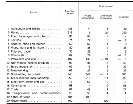
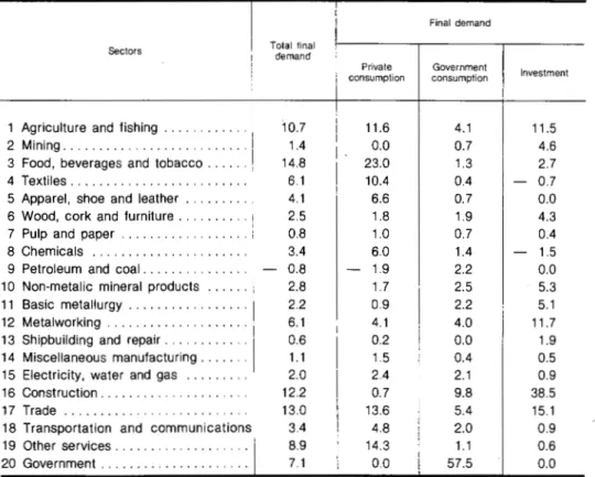
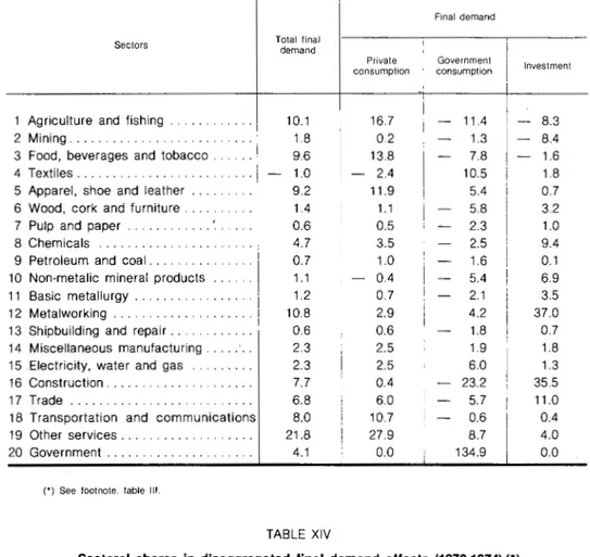
Concerning the sectoral structure of disaggregated final demand effects (tables XII, XIII and XIV), the following facts deserve to be mentioned.

Private consumption effects are mostly due to accrued demand for four types of suppliers of basic requirements.

TABLE X

Private consumption, Government consumption and investment effects (1964·1970) Percentage

Final demand

Sectors Total final

demand

Private _Investment

consumption

i

1 Agriculture and fishing ... ' _{66 81 - 2 - 12}

2 Mining ... -686 49 - 15 -720

3 Food, beverages and tobacco ... 68 73 - 2 - 2

4 Textiles ... - 18 - 30 5 7

5 Apparel, shoe and leather ... 78 76 1 1

6 Wood, cork and furniture ... 72 42 - 9 39

7 Pulp and paper ... 20 14

-

8 Chemicals ... 65 36 - 1 30

9 Petroleum and coal ... ... 42 44 - 3 1

10 Non-metalic mineral products ... 46

-

-

11 Basic metallurgy ... 62 24 - 3 41

12 Metalworking ... 64 13 1 50

13 Shipbuilding and repair ... 41 34 - 4 11

14 Miscellaneous manufacturing ... 57 45 1 10

15 Electricity, water and gas ... 65 52 5 8

16 Construction ... 104 4 - 9 109

17 Trade ... 148 97 - 4 55

18 Transportation and communications 101 100 0 1

19 Other services ... 82 78 1 3

TABLE XI

Private consumption, Government consumption and investment effects (1970·1974) Percentage

Finai demand

Total final

Seclors _demand

Private Government

Investment

consumption consumption

;

I

1 Agriculture and fishing ... i 108 71 5 32

2 Mining ... 318 6 21 290

3 Food, beverages and tobacco ... 90 84 1 4

4 Textiles ... 71 72 0 - 2

5 Apparel, shoe and leather ... -69 67 1 I 0

6 Wood, cork and furniture ... 80 35 7 38

7 Pulp and paper ... 35 26 4 5

8 Chemicals ... 67 72 3 - 8

9 Petroleum and coal ... 107 143

_-

10 Non·metalic mineral products ... 99 36 11 52

11 Basic metallurgy ... 63 16 8 39

12 Metalworking ... 68 27 5 35

13 Shipbuilding and repair ... 746 141 - 1 606

14 Miscellaneous manufacturing ... 259 216 I _{11 33}

15 Electricity, water and gas ... 77 57 10 10

16 Construction ... 98 4 10 85

17 Trade ... 67 42 3 21

18 Transportation and communications 58 50 4 4

19 Other services ... 104 100 2 2

20 Government ... 100 0 100 0

- - · - - -

-The first type comprises food in a broad sense. Agriculture and fishing and food, beverages, and tobacco benefited from consumptions effects at the tune of 1f3 of such effects in 1959-1964 and 1970-1974 and a little less

in 1964-1970.

The second type concerns textiles and apparel and shoe and leather, both with a somewhat erratic behaviour. Taking together those two sectors, their share in the three subperiods has been, respectively, 17 %, 9.5% and 4.6 %.

The third type is represented by trade and services with values around 30% in 1959-1964 and 1970-1974, but 34% in 1964-1970. However, while in the beginning ar.. in the end subperiods their relative shares have been quite similar, in the middle subperiod trade had no more than 6 % and services peacked to a 28 % share.

Government consumption effects are documented by the Government sector itself, thus reflecting the national accounts conventions adopted. Finally, regarding investment, there are two sectors which are the main beneficiaries of those effects: construction, with a share varying from 38 % in the initial subperiod to 29 % in the final period, and metalworking, with a maximum of 37 % in the middle subperiod and a minimum of 12 % in the initial one. These two opposed change$ are, to some extent, explained by the rising share of equipment in gross fixed capital formation as the structure of the economy grows in complexity. Apart from that, we must mention that trade has twice reached the 15 % mark in the initial and final periods and agriculture has once attained the share of 11.5 % in 1959-1964. Also chemicals, non-metallic mineral products and basic metallurgy usually account, individually, for more than 5 % of investment effects.

TABLE XII

Sectoral shares in disaggregated final demand effects (1959-1964) (*)

1

Sectors I _· Total final _demand

'

1 Agriculture and fishing ... · 2 Mining ...

·I

4 Textiles ... . 5 Apparel, shoe and leather ... . 6 Wood, cork and furniture ... , 7 Pulp and paper ... i

8 Chemicals ... .

9 Petroleum and coal ... .

10 Non-metalic mineral products ... I 11 Basic metallurgy ... I 12 M~tal~orking ...

1

13 Sh;pbwldmg and repa1r ...

1 .

14 Miscellaneous manufacturing ... .

15 Electricity, water and gas ... .

16 Construction ... .

17 Trade ... . 18 Transportation and communications I 19 Other services ... ·1

20 Government ... .

(') See footnote, table 111.

10.7 1.4 14.8 6.1 4.1 2.5 0.8 3.4 - 0.8 2.8 2.2 6.1 0.6 1.1 2.0 12.2 13.0 3.4 8.9 7.1

Final demand

Private Government consumption consumption

TABLE XIII

Sectoral shares in disaggregated final demand effects (1964·1970) (*)

Percentage

Final demand

Sectors Total final _demand

Private Government _Investment consumption consumption

I

1 Agriculture and fishing ...

.I

2 Mining ... ... 1.8 0.2 - 1.3 - 8.4

3 Food, beverages and tobacco ... . . I 9.6 13.8 - 7.8 - 1.6

4 Textiles ... _{. . . I -} 1.0 - 2.4 10.5 1.8

5 Apparel, shoe and leather 9.2 11.9 5.4 0.7

6 Wood, cork and furniture ... 1.4 1.1 5.8 3.2

7 Pulp and paper ... 0.6 0.5 - 2.3 1.0

8 Chemicals ... 4.7 3.5 2.5 9.4

9 Petroleum and coal ... ... 0.7 1.0 - 1.6 0.1

10 Non-metalic mineral products .... 1.1 I - 0.4 - 5.4 6.9

11 Basic metallurgy ... 1.2 0.7 - 2.1 3.5

12 Metalworking ... 10.8 2.9 4.2 37.0

13 Shipbuilding and repair ... 0.6 0.6 - 1.8 0.7

14 Miscellaneous manufacturing ... 2.3 2.5 1.9 1.8

15 Electricity, water and gas ... 2.3 2.5 6.0 1.3

16 Construction ... 7.7 0.4 - 23.2 35.5

17 Trade ... 6.8 6.0 - 5.7 11.0

18 Transportation and communications 8.0 10.7 - 0.6 0.4

19 Other services ... 21.8 27.9 8.7 4.0

20 Government ... 4.1 0.0 134.9 0.0

(•) See footnote. table Ill.

TABLE XIV

Sectoral shares in disaggregated final demand effects (1970·1974) (*)

Sectors

I _{Final demand} Total final

Sectors _demand

Private Government _Investment consl.<'mption consumption

i

:

10 Non-metalic mineral products ... j 2.4 0.8 - 0.1

I

5.5 11 Basic metallurgy ... . . . . . . 1.7 1.0

I 3.0 2.8

12 Metalworking _{. . . . . . . . . . . . . . .} i _{12.7 8.8 28.9 16.9}

i

13 Shipbuilding and repair ... 0.6 0.1 1.3

I 1.1

14 Miscellaneous manufacturing ... , 3.0 4.0 2.9 1.2

15 Electricity, water and gas ... 1.4 1.5 2.9 1.0

16 Construction ... . . . . . . . . . . . . . ' 10.5 0.3 0.9 28.6

17 Trade ... 14.7 15.2 4.7 15.2

18 Transportation and communications 4.1 6.6 _l 0.5 0.5

19 Other services ... ... 9.6 15.4

I

2.0 1.2

20 Government .. ... 2.8 0.0 55.9 _I 0.0

-

-(•) See footnote, table Ill.

6 - Conclusions

According to the Torii-Fukasaku methodology, private consumption changes have been the dominant source of output growth in every subperiod. Moreover, its share rose consistently along the period.

Other components of final demand, namely Government consumption, fully reflected the consequences of resources mobilization in response to Salazar and Caetano's colonial war policies. Investment uses, although severely affected in the mid 60's, increased their importance in the early 70's. The report has also shown that movements towards a much more open economy have to be evaluated taking into account both export and import substitution effects. In the 60's, and on an aggregated basis, the overall balance improved at a reasonable pace. Its share in total output growth increased from 18.1% in 1959-1964 to 21.5% in 1964-1970, both aggregate exports and import substitution effects being positive.

However, in 1970-1974 the net foreign effects experienced a sharp drop, to 11.2 %. In this subperiod, aggregate import substitution effects varied from little less than

+

A comment is also in order, regarding methodology. Other methods of measurement are available. To what extent will the broad picture change if we apply alternative methods? Finally, what can we gain if we take a finer sectoral detail?