Ricardo Lourenço-de-Moraes1,2,3*, Felipe S. Campos4,5, Rodrigo B. Ferreira6, Karen H. Beard7, Mirco Solé8, Gustavo A. Llorente4, Rogério P. Bastos3
1Programa de Pós-graduação em Ecologia e Monitoramento Ambiental (PPGEMA), Universidade Federal da Paraíba (UFPB), Campus IV, Litoral Norte, Av. Santa Elizabete s/n, Centro, 58297-000, Rio Tinto, PB-Brazil
2Programa de Pós-graduação em Ecologia de Ambientes Aquáticos Continentais (PEA), Universidade Estadual de Maringá, Av. Colombo 5790, Bloco G-90, 87020-900, Maringá, PR, Brazil
3Laboratório de Herpetologia e Comportamento Animal, Universidade Federal de Goiás, Campus Samambaia, 74690-900, Goiânia, GO, Brazil
4Departament de Biologia Evolutiva, Ecologia i Ciències Ambientals, Facultat de Biologia, Universitat de Barcelona, 08028, Barcelona, Spain
5NOVA Information Management School (NOVA IMS), Universidade Nova de Lisboa, Campus de Campolide, 1070-312 Lisboa, Portugal
6Laboratório de Ecologia da Herpetofauna Neotropical, Programa de Pós-graduação em Ecologia de Ecossistemas,Universidade Vila Velha, 29102-920, Vila Velha, ES, Brazil
7Department of Wildland Resources and the Ecology Center, Utah State University, 84322-5230, Logan, UT, USA
8Departamento de Ciências Biológicas, Universidade Estadual de Santa Cruz, 45662-000, Ilhéus, BA, Brazil
This is the peer reviewed version of the following article: Lourenço‐de‐Moraes, R, Campos, FS, Ferreira, RB, et al. Functional traits explain amphibian distribution in the Brazilian Atlantic Forest. J Biogeogr. 2019; 00: 1– 13. https://doi.org/10.1111/jbi.13727. This article may be used for non-commercial purposes in accordance with Wiley Terms and Conditions for Use of Self-Archived Versions."
This work is licensed under a Creative Commons Attribution-NonCommercial 4.0 International License.
Functional traits explain amphibian distribution in the Brazilian Atlantic Forest
1 2
Ricardo Lourenço-de-Moraes1,2,3*, Felipe S. Campos4,5, Rodrigo B. Ferreira6, Karen H. 3
Beard7, Mirco Solé8, Gustavo A. Llorente4, Rogério P. Bastos3 4
5
1Programa de Pós-graduação em Ecologia e Monitoramento Ambiental (PPGEMA), 6
Universidade Federal da Paraíba (UFPB), Campus IV, Litoral Norte, Av. Santa 7
Elizabete s/n, Centro, 58297-000, Rio Tinto, PB-Brazil 8
2Programa de Pós-graduação em Ecologia de Ambientes Aquáticos Continentais (PEA), 9
Universidade Estadual de Maringá, Av. Colombo 5790, Bloco G-90, 87020-900, 10
Maringá, PR, Brazil 11
3Laboratório de Herpetologia e Comportamento Animal, Universidade Federal de 12
Goiás, Campus Samambaia, 74690-900, Goiânia, GO, Brazil 13
4Departament de Biologia Evolutiva, Ecologia i Ciències Ambientals, Facultat de 14
Biologia, Universitat de Barcelona, 08028, Barcelona, Spain 15
5NOVA Information Management School (NOVA IMS), Universidade Nova de Lisboa, 16
Campus de Campolide, 1070-312 Lisboa, Portugal 17
6Laboratório de Ecologia da Herpetofauna Neotropical, Programa de Pós-graduação em 18
Ecologia de Ecossistemas,Universidade Vila Velha, 29102-920, Vila Velha, ES, Brazil 19
7Department of Wildland Resources and the Ecology Center, Utah State University, 20
84322-5230, Logan, UT, USA 21
8Departamento de Ciências Biológicas, Universidade Estadual de Santa Cruz, 45662-22
000, Ilhéus, BA, Brazil 23
24
*Correspondence: Ricardo Lourenço-de-Moraes; Programa de Pós-graduação em 25
Ecologia e Monitoramento Ambiental (PPGEMA), Universidade Federal da Paraíba, 26
Campus IV, Litoral Norte Av. Santa Elizabete s/n, Centro, 58297-000, Rio Tinto, PB, 27
Brazil 28
Email: [email protected]; Phone: +(55)4432381821; Fax: 29 (+55)4432381821 30 31 ACKNOWLEDGEMENTS 32
RLM, RPB, and RBF thank Conselho Nacional de Desenvolvimento Científico e
33
Tecnológico for scholarships (140710/2013-2; 152303/2016-2; 430195/2018-4) and 34
research productivity. This study was financed in part by the Coordenação de 35
Aperfeiçoamento de Pessoal de Nível Superior - Brasil (CAPES) - Finance Code 001 36
(FSC 99999.001180/2013-04). We thank the ComissãoTécnico-Científica do Instituto 37
Florestal, Estado de São Paulo (COTEC), Instituto Ambiental do Paraná- Estado do 38
Paraná (IAP), and the Instituto Chico Mendes de Conservação da Biodiversidade for 39
logistical support and collection licenses (ICMBio/SISBIO 30344 and 44755). 40
Abstract
41
Aim: Species distributions are one of the most important ways to understand how
42
communities interact through macroecological relationships. The functional abilities of 43
a species, such as its plasticity in various environments, can determine its distribution, 44
species richness, and beta diversity patterns. In this study, we evaluate how functional 45
traits influence the distribution of amphibians, and hypothesize which functional traits 46
explain the current pattern of amphibian species composition. 47
Location: Atlantic Forest, Brazil.
48
Methods: Using potential distributions of Brazilian Atlantic Forest of amphibian
49
species and based on their functional traits, we analysed the influence of biotic and 50
abiotic factors on species richness, endemism (with permutation multivariate analysis), 51
and beta diversity components (i.e. total, turnover and nestedness dissimilarities). 52
Results: Environmental variables explained 59.5% of species richness, whereas
53
functional traits explained 15.8% of species distribution (geographical species range) 54
for Anuran and 88.8% for Gymnophiona. Body size had the strongest correlation with 55
the species distribution. Results showed that species with medium to large body size, 56
and species that are adapted to living in open areas tended to disperse from west to east 57
direction. Current forest changes directly affected beta diversity patterns (i.e. most 58
species adapted to novel environments increase their ranges). Beta diversity partitioning 59
between humid and dry forests showed decreased nestedness and increased turnover by 60
increasing altitude in the southeastern region of the Atlantic Forest. 61
Main conclusions: Our study shows that functional traits directly influence the ability
62
of the species to disperse. With the alterations of the natural environment, species more 63
apt to these alterations have dispersed or increased their distribution, which 64
consequently changes community structure. As result, there is nested species 65
distribution patterns and homogenization of amphibian species composition throughout 66
the Brazilian Atlantic Forest. 67
68
KEYWORDS
69
Anura, beta diversity partitioning, conservation, functional abilities, Gymnophiona, 70
spatial distribution 71
INTRODUCTION
73
Distribution patterns, dispersion processes and permanence of species are some of the 74
most studied topics by ecologists and biogeographers. The distribution of organisms is 75
the basis of ecological studies and can be determined by biotic and abiotic factors 76
(Hutchinson, 1957; Soberón, 2007). For example, current patterns of species 77
distributions are linked to historical and contemporary dispersals influenced by species 78
characteristics and their specific functional traits (Ricklefs, 1987; Oberdorff et al., 1997; 79
Svenning & Skov, 2007; Carnaval & Moritz, 2008; Carnaval et al., 2009; Baselga et al., 80
2012; Silva et al., 2014). On the other hand, habitat characteristics influence the spatial 81
and temporal distributions of species (Hawkins, 2001; Ferreira et al., 2016; Figueiredo 82
et al., 2019). Thus, historical dispersal can be understood using environmental data of 83
the localities at which species have been recorded and the geographical boundaries that 84
restrict them (Gaston, 1991). 85
Because ectothermic species are largely limited by climatic zones (Pfrender et 86
al., 1998), both dispersal limitation and climate variation can be critical determinants of 87
species ranges (Baselga et al., 2012; Lourenço-de-Moraes, Lansak-Tohâ et al., 2019). 88
Further, the distribution of a species is often related to species characteristics, such as 89
body size and local abundance (Brown & Maurer, 1989; Gaston, 1990; Lawton, 1993). 90
For example, small ectothermic species can dehydrate faster than large species 91
(MacLean, 1985), and many are prey to vertebrates and invertebrates (Toledo et al., 92
2007; Wells, 2007). Thus, ectotherms rely upon their morphological and physiological 93
adaptations to succeed in surviving and dispersing. In this sense, understanding 94
functional traits (Jimenez-ValVerde et al., 2015) may be key to understanding the 95
potential distribution of the ectotherms (Díaz et al., 2007; Gómez-Rodrigues et al., 96
2015). 97
Amphibian species richness is non-random process and is often related to 98
temperature and precipitation (Casemiro et al., 2007; Vasconcelos et al., 2010). The 99
sites of high species richness can provide species for sites of low species richness (i.e. 100
metacommunity theory; Leibold & Mikkelson, 2002; Ulrich & Gotelli, 2007; Baselga, 101
2010; Lourenço-de-Moraes, Malagoli et al., 2018). Geographical distributions of 102
amphibians are strongly affected by type of habit, as terrestrial and aquatic preferences 103
of juveniles and adults, and their ability to disperse across the landscape (Patrick et al., 104
2008). Microclimate characteristics of habitat as forests and open areas can provide 105
physiological and ecological constraints for many species because they influence 106
forage, reproduction and survival (Huey, 1991). Such constraints strongly affect the 107
causes and consequences of dispersal abilities as well as the nature of species 108
interactions (McGill et al., 2006), including reproductive modes, activity time and 109
antipredator mechanisms (Monkkonen & Reunanen, 1999; Fahrig, 2001; Ferreira et al., 110
2019). Given that short-term impacts of habitat loss increase with dispersal ability of 111
amphibians (Homan et al., 2004), there is a critical need to investigate the spatial 112
mismatches between the distribution of species and environmental changes under 113
functional-traits approaches (Cushman, 2006; Berg et al., 2010). Forest isolation is a 114
critical factor in biological community structure and fundamentally important in a 115
habitat fragmentation context (Dixo et al., 2009). Understanding beta diversity patterns 116
and evaluating their different compositions (i.e. turnover or nestedness components) 117
along a latitudinal and longitudinal gradient can be an important tool for understanding 118
the dispersal processes of these species (Baselga, 2008, 2010). 119
Knowing that amphibians are dispersal limited due to their morphological, 120
physiological and ecological characteristics (Richter-Boix et al., 2007), we evaluated 121
the species richness (correlated to environmental variables) and beta diversity (turnover 122
and nestedness) of amphibians in the Atlantic Forest, while assessing their potential 123
dispersal based on functional traits. In this context, species typical of open areas can 124
benefit from the alteration of forests due to the increase of their habitat area; and smaller 125
species should be more associated with areas with milder temperatures (e.g. areas of 126
high altitude) due to lower water loss rate to the environment. In this study, we tested 127
the hypothesis that functional traits explain the current pattern of amphibian species 128
composition in the Atlantic Forest. Depending on the functional trait (e.g. body size and 129
ecological specializations) the species may have more ability to disperse and increase its 130
distribution. 131
132
MATERIALS AND METHODS
133
Study region
134
The Brazilian Atlantic Forest has a latitudinal range extending into both tropical and 135
subtropical regions (Myers et al., 2000). The longitudinal range extends from the coast 136
to 1,000 km inland, and the altitudinal range extends from 0 to 2000 m a.s.l. (Cavarzere 137
& Silveira, 2012). Originally, this biome covered around 150 million ha with a wide 138
range of climatic belts and vegetation formations (Tabarelli et al., 2005; Ribeiro et al., 139
2009). Currently only about 12% of the original biome remains (Ribeiro et al., 2009). 140
This biome occurs across 14 states from the south to the northeast of Brazil (Fig. 1). To 141
test the hypothesis that functional traits explain the current pattern of amphibian species 142
composition (see Appendix 1, Fig 1.1) and understand the pattern of beta diversity in 143
each study sites, we analysed differences in species compositions (richness and 144
endemism) and mapped out potential dispersal routes. We delimitated the study sites in 145
relation to: i) geomorphological barriers (see Dominguez et al., 1987; Bittencourt et al., 146
2007); ii) abiotic barriers (Worldclim database; see below); iii) forest composition 147
barriers (see Olson et al., 2001); iv) names based in political divisions; and v) size of 148
area. 149
Given that each state has different environmental laws (e.g. IAP-Instituto 150
Ambiental do Paraná- Paraná state, COTEC - ComissãoTécnico-Científica do Instituto 151
Florestal, São Paulo state, INEMA - Instituto do Meio Ambiente e Recursos Hídricos, 152
Bahia state), we used spatial data that allow different conservation strategies at local 153
scales (i.e. environmental state policies). Two states have all of their territory included 154
in determining the composition of species, RJ (Rio de Janeiro) and ES (Espírito Santo), 155
due to their smaller sizes, similar forest composition and abiotic features. Four states 156
have all of their territory separated into eastern and western sections, because they are 157
large and have different forest composition (eastern rain forest, western seasonal forest): 158
EPR (eastern Paraná),WPR (western Paraná), ESC (eastern Santa Catarina),WSC 159
(western Santa Catarina), ERS (eastern Rio Grande do Sul),WRS (western Rio Grande 160
do Sul); and the “SMGM” refers to four connected states in seasonal forests (includes 161
western of São Paulo-S, north Mato Grosso do Sul-M, south Goiás -G and extreme 162
south Minas Gerais - M);MS refers to the south-western Mato Grosso do Sul . The 163
Pernambuco, Sergipe, Ceará, Paraíba and Rio Grande do Norte states were included in 164
region N (Northeast), due to their smaller territories inside this biome, and similar forest 165
composition and abiotic features. We also separated two states in regions north and 166
south, due to their large territory, and different forest composition and abiotic features – 167
SBA (south Bahia), NBA (north Bahia), SMG (south Minas Gerais) and NMG (north 168
Minas Gerais). In total, we assessed 16 study sites (see Fig. 2). 169
170
Species distribution data
171
We included species occurrence records available through the Global Biodiversity 172
Information Facility (GBIF: http://www.gbif.org), and added range maps of each 173
species from the IUCN Red List of Threatened Species (IUCN, 2017: 174
http://www.iucnredlist.org/technical-documents/spatial-data). In addition, we conducted 175
acoustic and visual nocturnal/diurnal amphibian survey (Crump & Scott Jr., 1994; 176
Zimmerman, 1994) in 11 Protected Areas (PAs), from the southern to the northeastern 177
Brazil (see Appendix 1, Fig. 1.2). We followed Frost (2019) for the amphibian 178
nomenclature with exception of the species synonymized as Allobates olfersioides 179
which we consider to be distinct species (A. olfersioides, A. alagoanus and A. capixaba 180
see Forti et al., 2017). 181
We used ArcGIS 10.1 software (ESRI, 2011) to build presence/absence matrices 182
from the species distribution data by superimposing a grid system with cells of 0.1 183
latitude/longitude degrees, creating a network with 10,359 grid cells. We used the 184
“Spatial Join” ArcGIS toolbox to transform species' spatial occurrences in matrices, 185
matching rows from the join features to the target features based on their relative spatial 186
locations. Then, we combined vector files based on expert knowledge of the species' 187
ranges and forest remnant polygons into an overall coverage for species distribution 188
modelling. We only considered spatial occurrences by those species where the 189
distribution data intersected at least a grid cell. We used forest remnant data to meet the 190
habitat patch requirements based on visual interpretation at a scale of 1:50,000, 191
delimiting more than 260,000 forest remnants with a minimum mapping area of 0.3 192
km2. Therefore, we considered a species present in a cell if its spatial range intersected 193
more than 0.3 km2. We also used the “Count Overlapping Polygons” ArcGIS toolbox to 194
obtain the species richness at the spatial resolution assessed, removing all duplicate 195
records from the analyses (i.e. repeated records of a species at a single locality). 196
197
Environmental variables
198
We took the mean of six environmental variables for each grid cell, which included one 199
topographic (altitude), one biotic (tree cover) and four climatic variables (annual 200
precipitation, mean annual temperature, annual evapotranspiration, and net primary 201
productivity). We obtained altitude, annual precipitation and mean annual temperature 202
from the WorldClim database at 0.05º spatial resolution (http://www.worldclim.org/). 203
We obtained annual evapotranspiration (AET) from the Geonetwork database 204
(http://www.fao.org/geonetwork/srv/); net primary productivity (NPP) from the 205
Numeral Terra dynamic Simulation Group (http://www.ntsg.umt.edu/data), and tree 206
cover from Global Forest Change 2000-2014 database 207
(http://earthenginepartners.appspot.com/science-2013-global-208
forest/download_v1.2.html). All of these variables are known to represent either 209
potential physiological limits for amphibians or barriers to dispersal (Vasconcelos et al., 210
2010; Silva et al., 2012). We drew maps using the ArcGis10.1 software (ESRI, 2011). 211
212
Functional traits
213
We characterized the functional traits of 531 amphibian species using Haddad et al. 214
(2013), ecological information from the IUCN database, scientific literature on the 215
original descriptions of the species, and data from our fieldwork (see Appendix 1, Table 216
1.1). We set out the following functional traits: body size, reproductive mode (subtraits: 217
direct or indirect), habitat (subtraits: forested areas, open areas, and both), activity time 218
(subtraits: nocturnal, diurnal, and both), toxicity (subtraits: toxic, unpalatable or bad 219
odour, and non-toxic), and habit (subtraits: arboreal, phytotelmate, terrestrial, cryptic, 220
fossorial, rheophilic, semi-aquatic, and aquatic). The subtraits terrestrial (on the ground 221
or in the leaf litter on the forest floor) and cryptic (hidden in galleries, crevices or in 222
natural or excavated holes in the ground and ravines or under the leaf litter) were 223
included because they are important characteristics which generate different patterns of 224
geographical dispersion. All these functional traits interact (directly or indirectly) in the 225
ecosystem functioning (Duellman & Trueb, 1994; Wells, 2007; Toledo et al., 2007; 226
Haddad et al., 2013; Hocking & Babbitt, 2014). See Appendix 1, Table 1.2 for more 227
details about the specific functions and the ecosystem supporting services of each one of 228 these traits. 229 230 Data Analyses 231
Effect of environmental variables on species richness and endemic species
232
We evaluated the response of species richness and endemic species separately to the 233
predictor variables: altitude (minimum/maximum elevation), mean annual precipitation 234
(MAP), mean annual temperature (MAT), mean annual evapotranspiration (MAE), net 235
primary productivity (NPP), and tree cover (TC). We used the term endemic species for 236
species that occur in only one of the 16 study site (see Fig. 2), and calculated endemic 237
and richness species for each grid cell of 0.1º (10,359 cells). For these analyses, we used 238
permutation multivariate analysis of variance (PERMANOVA), with 1,000 239
permutations based on a Euclidean distance matrix through the “adonis” function of the 240
package “vegan” (Oksanen et al., 2013), in the R software (R Development Core Team, 241
2017). 242
243
Effects of functional trait body size in the species richness
244
We used simple linear models to test the relationship between body size (original body 245
size of each species) on species richness across Atlantic Forest. For this, we calculated 246
mean body size for each grid cell. Then, we evaluated the relationship between mean 247
body size, and latitude, longitude and altitude. We performed these analyses using the 248
package 'vegan' (Oksanen et al., 2013) in the R software (R Development Core Team, 249
2017). 250
251
Effects of functional traits in geographical distribution of species
252
First, we calculated the geographical range of each species to the predicted body size, 253
toxicity, reproductive mode, habit, habitat and activity time for Anura and body size, 254
reproductive mode, habitat and habit for Gymnophiona. For this, we used permutation 255
multivariate analysis of variance (PERMANOVA), with 1,000 permutations. 256
Second, we used Boxplots (categorized – miniature <2cm, small ≥ 2 and <3cm, 257
medium ≥3 and < 8cm, large ≥8cm) and percentage histograms to visualize the traits 258
that better explained species distribution. We analysed the differences between the traits 259
separately for anurans (ANOVA) and gymnophionas (Kruskal-Wallis), depending on 260
normality using the Shapiro test (parametric and non-parametric data). We performed 261
these analyses separately due to lack of information on Gymnophiona and their different 262
characteristics of ecological traits and body size (Haddad et al., 2013). We calculated 263
these analyses for each grid cell, using the R packages 'vegan' (Oksanen et al., 2013),
264
'car' (Fox & Weisberg, 2011), 'FSA' (Ogle, 2016), and 'lattice' (Sarkar, 2008) in the R 265
software (R Development Core Team, 2017). 266
267
Similar geographical species groups
268
First, we examined whether there was independence of spatial correlation of species 269
composition among the 16 study sites (matrix of spatial data vs. matrix of species 270
composition, Euclidean distance matrix). For this, we used Pearson correlation tests 271
using the Mantel with 1,000 permutation (Legendre & Legendre, 1998). Second, we 272
used a similarity measure (i.e. Euclidean distance matrix) of the 16 study sites to rank 273
the groups of similar species composition. Ordination of the 16 study sites was based on 274
this faunal dissimilarity matrix, which was submitted to a nonparametric 275
multidimensional scaling analysis (NMDS, Legendre & Legendre, 1998) and the most 276
likely solution was evaluated by Pearson correlation. The calculation of the variance is 277
captured by a regression matrix from the original distances (Bray-Curtis) and the final 278
array distances (Euclidean) (Fig. 2b). Third, we draw a dendrogram by taking Euclidean 279
distance as the measure of resemblance and average linkage procedure as the linkage 280
rule (Fig. 2c). We performed these tests using the package 'vegan' (Oksanen et al., 2013) 281
in the R software (R Development Core Team, 2017). 282
283
Beta diversity measures
284
First, we used two complementary metrics for beta diversity analysis by considering 285
species presence and absence. To determine if the pattern among anuran communities is 286
nested, we calculated a nestedness metric based on overlap and decreasing fill (index 287
NODF) of Almeida-Neto et al. (2008) and Ulrich et al. (2009) across the 16 study sites 288
(Fig. 2a). The matrix is decreasing for both columns and rows; columns ranked the 289
areas according to their species richness and rows ranked the species from, the most 290
frequent to the rarest. With this approach, we create and order study sites as major biota 291
and its subsets biota. To perform this analysis, original matrices were submitted to 292
1,000 simulations. We performed this analysis for all localities separately using the 293
package 'vegan' (Oksanen et al., 2013) in the R software (R Development Core Team, 294
2017). 295
Second, we conducted beta diversity partitioning and computed distance 296
matrices using pairwise dissimilarities βsor (i.e. measure total beta diversity), βsim (i.e. 297
measure spatial turnover), and βnes (i.e. measure nestedness) (Baselga, 2010). We 298
computed these analyses among the 16 study sites to show the directions of the species 299
distributions. We considered larger nesting values means more species similar to the 300
area of major species richness, and larger numbers of turnover means less similar 301
species composition. We follow the sequence provided by NODF for analysis of beta 302
diversity partitioning. This method partitions the pairwise Sørensen dissimilarity 303
between two communities (βsor) into two additive components accounting for species 304
spatial turnover (βsim) and nestedness-resultant dissimilarities (βsne). Since βsor and 305
βsim are equal in the absence of nestedness, their difference is a net measure of the 306
nestedness-resultant component of beta diversity, so βsne = βsor – βsim (Baselga, 307
2010). 308
Third, to available the effects of topographic variation among the 16 study sites 309
and species composition, we ran the analyses using four approaches: i) entire altitudinal 310
range (0-2000m a.s.l.); ii) 0-300m a.s.l.; iii) 300-700m a.s.l.; iv) 700-2000m a.s.l.. We 311
performed these tests using the package 'betapart' (Baselga & Orme, 2012) in the R 312
software (R Development Core Team, 2017). 313
314
RESULTS
315
We found that the environmental variables explained 59.5% of the amphibian species 316
richness across Atlantic Forest. Temperature-MAT was the main variable (39.3%), 317
followed by precipitation-MAP (11.4%), and net primary productivity-NPP (8.6%) 318
(Appendix 2, Table 2.1). For study sites with endemic amphibian species, the 319
environmental values explained 26% of the endemism, of which temperature was the 320
main variable (22%), followed by altitude (2%) (Appendix 2, Table 2.2). 321
For Anura, changes in functional traits explained 15.8% of the species 322
distribution (geographical species range). Habitat was responsible for about 9%, body 323
size 3%, habit 1% and toxicity 0.8% of the variation in the species distribution. 324
Reproductive mode and activity time traits did not show any significant relationship to 325
species distribution (Appendix 2, Table 2.3). 326
For Gymnophiona, two main traits explained 88.8% of the species distribution. 327
Habitat was responsible for about 67.4% and reproductive mode 15.7% of the variation 328
in the species distribution patterns. The body size and habit traits did not show any 329
relationship to species distribution (Appendix 2, Table 2.4). 330
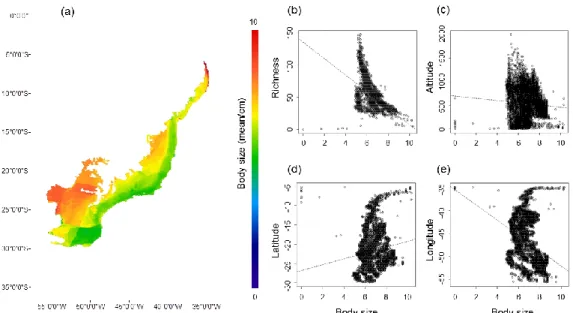
For Anura and Gymnophiona, the trait body size showed low but significant 331
correlations with species richness (r2 = 0.398; p < 0.001), longitude (r2 = 0.103; p < 332
0.001), latitude (r2 = 0.025; p < 0.001), and altitude (r2 = 0.006; p < 0.001). Medium to 333
larger species are more abundant in the region west (lower longitudes) and extreme 334
north (higher latitudes) in the Atlantic Forest (Fig. 3). Medium to smaller species are 335
more abundant in the region east (lowerlatitudes and higher altitudes) in the Atlantic 336
Forest (Fig. 3). 337
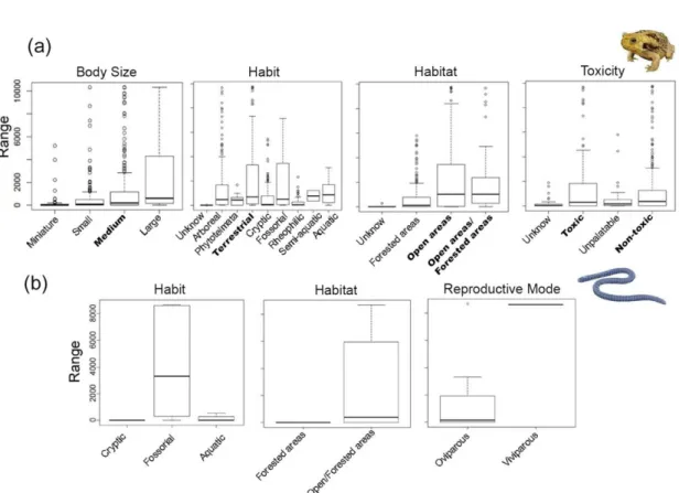
For the functional subtraits, the largest distribution distances in Anura (p < 0.05) 338
was found between species of open areas and species of open/forested areas, species of 339
medium body size, terrestrial, and toxic and non-toxic species (Appendix 2, Table 2.5 340
and Fig. 4a). The subtraits in Gymnophiona are non-significant (p > 0.05) (Appendix 2, 341
Table 2.6 and Fig. 4b), but 35% of species of open/forested areas are distributed in more 342
than 2,000 range cells, and 100% of viviparous species are distributed in more than 343
6,000 range cells (Appendix 2, Fig. 2.2). 344
The Mantel tests indicated spatial correlation of species composition and 345
geographical distance among the 16 study sites (r2 = 0.30, p = 0.019). The dendrogram 346
used the scores of the NMDS axis (7 dimensions, r2 = 0.99, p > 0.001) and showed the 347
presence of three groups of similar composition in the Atlantic Forest (Fig. 2b). The 348
major species richness was in group 1 (ESP, RJ and SMG), characterized by humid 349
forests with high species richness and endemism. Group 2 was divided into two 350
subgroups: one formed by MS, WPR, WSC, WRS and SMGM (subgroup 2a), through 351
seasonally dry forests with low species richness and endemism, and another one formed 352
by EPR, ESC and ERS (subgroup 2b), through humid forests with presence of 353
Araucarias forest. The group 3 was formed by ES, NMG, SBA, NBA and N and has 354
high temperature and low or no seasonality (Appendix 2, Fig. 2.3). 355
Our results of the NODF values indicated significant nestedness (NODF = 38.7, 356
p < 0.001), showing the sites ESP, RJ and SMG as the major biota (Fig. 2a). The beta
357
diversity partitioning revealed that the highest values were between groups 1 and 3 358
(βsor mean 0.684 ± 0.093) followed by the group 2a (βsor mean 0.675 ± 0.126). Among 359
group 3, the values increase by increasing the difference in species composition 360
according to altitude, decreasing βsim and increasing βnes; wherein the area N has 361
highest βnes (0.281) among the species that occur 700-2000 m a.s.l., and the area SBA 362
has highest values of βsim (0.582) among the species composition that occur in 300 m 363
a.s.l. (Appendix 2, Table 2.6 and Fig. 5). 364
There is a similar pattern among species from the group 2a. However, the βnes 365
decreases and βsim decreases then increases slightly at higher altitudes, wherein the 366
area MS has highest values of βnes (0.669) whereas that area WRS has highest values 367
of βsim (0.397) both among species which occur between 300-700 m a.s.l.. Among the 368
groups 1 and 2b the values of βsor increases abruptly with increasing altitude (βsor 369
mean 0.215-0.609). The main difference in this value of βsim (0.353-0.395) increases 370
according to increasing the differences in the species composition between altitudes. 371
The area ERS had the highest value of βnes (0.281) among the species that occur from 372
700-2000 m a.s.l. and the highest value of βsim (0.480) among the species that occur 373
300-700m a.s.l. (Appendix 2, Table 2.6 and Fig. 5). 374
The differences between the compositions were among the species that occur in 375
the lowland (0-300 m) and hilltops (700-2000 m). Between the groups 1 and 2a, 376
nestedness decrease with increasing altitude and increasing turnover between 700-2000 377
m and 0-300 m altitude. Between the groups 1 and 2b, nestedness decrease and 378
increased composition turnover with increasing elevation, which has a slight increase in 379
beta diversity pattern between species that occur in 300-700 m altitude. Between groups 380
1 and 3 nestedness increases and then decreases gradually by increasing altitude, 381
increasing turnover pattern. The group 2b indicates higher endemism rate on the 382
mountainous region, whereas the group 3 in the higher endemism rate on lowlands 383 (Fig.5). 384 385 DISCUSSION 386
Effect of environmental variables on species richness and endemic species
387
Our results showed that mean annual temperature has the greatest influence on 388
amphibian richness and endemic species in the Atlantic Forest. Due to their 389
physiological characteristics, amphibians are dependent of humidity and mild 390
temperatures (Wells, 2007; Crump, 2010). We also found correlations between species 391
richness and precipitation, corroborating other related studies (Casemiro et al., 2007; 392
Ortiz-Yusty et al., 2013; Vasconcelos et al., 2014). The correlation of species richness 393
with NPP and natural forest formations were also strongly correlated to rainfall (Rueda 394
et al., 2010). High altitudes have a higher number of endemic species due to the lower 395
temperatures and higher humidity (Cruz & Feio, 2007). However, lowland areas with 396
the same features (i.e. milder temperatures and higher humidity) also have endemic 397
species, and this may be related to historical events (Carnaval et al., 2012). 398
Due to high humidity and diversity of microhabitats, many Neotropical 399
amphibians evolved to be small (Rittmeyer et al., 2012). These species are more 400
susceptible to humidity loss (MacLean, 1985; Ashton, 2001) and many are restricted to 401
conserved forests to maintain their environmental favourability (Lourenço-de-Moraes et 402
al., 2014; Ferreira et al., 2016); such as areas of milder temperatures, higher rainfall, and 403
higher vegetation cover. Our results showed that amphibians in areas with lower 404
latitudes, intermediary longitudes and high altitudes tend to have smaller body sizes 405
species. Therefore, we highlight relationships between species richness and body size 406
that directly relate to environmental conditions. This may lead to restricted gene flow 407
between populations and accelerate genetic differentiation (Pabijan et al., 2012). 408
Consequently, it may have limited these species to rainforests where such genetic 409
differentiation is most commonly observed (Rodríguez et al., 2015), and these factors 410
may have contributed to the large number of small species (Lourenço-de-Moraes, Dias 411
et al., 2018). 412
413
Effects of functional traits in geographical distribution of species
414
We showed that amphibian species (especially anurans) with the widest distribution are 415
adapted to live in open areas, have medium body size, and are terrestrial and toxic. In 416
our study, species with the medium to large body size have better dispersal abilities, 417
such as Odontophrynus americanus (family Odontophrynidae), Leptodactylus 418
mystacinus (family Leptodactylidae) and Rhinella diptycha (family Bufonidae) (Haddad
419
et al., 2013). Species as L. mystacinus, with the same characteristics except toxicity also 420
have wide distributional ranges due to distinct factors that may improve their range 421
expansion (e.g. physiological, behavioural, and morphological traits). For example, 422
species with a variety of antipredator mechanisms may be more likely to avoid a wider 423
range of predators (Lourenço-de-Moraes et al., 2016), that allows successful dispersal. 424
In addition, species from open areas with larger ranges also occur in drier biomes, such 425
as the Cerrado and the Caatinga. 426
Our findings revealed that the distributions of Atlantic Forest amphibians are 427
related to their functional traits, of which the habitats comprising open areas can favour 428
larger species better adapted to high temperatures and low humidity rates. Most of the 429
species that occur in the Atlantic Forest has body size less than 30 mm, losing water 430
more quickly to the environment (MacLean, 1985). In addition, the type of habitat 431
preference may be determinant for the species distribution (Gouveia & Correia, 2016). 432
Because of this, even small arboreal species, such as Dendropsophus nanus and D. 433
minutus, have a greater ability to dispersal due to their ability to occur in open areas
434
(Haddad et al., 2013). However, small and miniature species with wide distribution, 435
such as D. minutus and Pseudopaludicola falcipes are species complexes; and thus their 436
current distribution may be overestimated (Gehara et al., 2014; Langone et al., 2016). 437
Many open area species are expanding or expanded their ranges due to forest 438
destruction (e.g. Leptodactylus fuscus). Habitat is an important trait for dispersal in an 439
environment transformed into open areas. However, species of open areas are not found 440
in forests, or they are found in low abundance (Campos & Lourenço-de-Moraes, 2017; 441
author's pers. obs.), therefore, we suggest that these species are not generalists, but 442
specialists of open areas and opportunistic. 443
444
Beta diversity patterns We revealed a homogenized pattern of species in Atlantic
445
Forest, which can be explained by beta diversity (NODF nestedness). Species of open 446
areas tend to disperse from west to east due to deforestation. The mountains of Serra do 447
Mar and Mantiqueira can be limiting geographical barriers for small amphibians 448
restricted to forest habits (Haddad, 1998; Morellato & Haddad, 2000). Moreover, the 449
geographical barrier Rio Doce divides the region ES and part of NMG (Bates et al., 450
1998; Costa et al., 2000) and influences dispersal and composition of species from the 451
group 3. ES has southern (group 1) and northern (group 3) species of the Atlantic 452
Forest, while NMG is more related to northern (group 3) species. Few strictly forest 453
species have large ranges in the Atlantic Forest. Haddadus binotatus is a forest species 454
that is widely distributed in the Atlantic Forest. This species may have dispersed 455
through drier forests in the western region or during the Glacial period due to ocean 456
regression (Atlantic Forest hypothesis, see Leite et al., 2016). However, it is possible 457
that this is a species complex (Dias et al., 2011) and the current distribution of these 458
species may be overestimated. 459
. 460
Our results indicate changes in beta diversity pattern between hilltops and 461
lowland, the nestedness pattern decreasing with increasing altitude and increasing the 462
turnover. This biogeographic difference in species compositions according to 463
topographic location is a non-random pattern; temporal and environmental processes 464
influenced this pattern (Carvalho, 2010). Different altitudes (0-2000m) have different 465
degrees of environmental variations that determine amphibian composition. 466
Mountainous areas and geological events create important biogeographic barriers 467
(Haddad et al., 1998; Costa et al., 2000), and generate vicariance processes (Almeida & 468
Santos, 2010). Consequently, high altitude areas (i.e. Serra do Mar, Cruz & Feio, 2007) 469
and natural lowland forests (i.e. south Bahia, Mira-Mendes et al., 2018) have high 470
species diversity and endemism reflecting the turnover pattern. The nestedness pattern is 471
generated by species with functional traits that allow dispersal between sites. . 472
According to our findings, it is possible to separate the Atlantic Forest into three 473
major regions of endemism. Our results point to groups 1, 2b and 3 as the areas with the 474
highest rates of endemic and rare species. The beta diversity values corroborate the 475
hypothesis of endemism during the Pleistocene glacial (Carnaval et al., 2009; Carnaval 476
et al., 2014) and Anthropocene (Lourenço-de-Moraes, Campos et al., 2019). The two 477
extremes of this biome (i.e. southern and northern most) have higher turnover rates 478
compared to group 1. Group 3 has shared genera with the Amazon forest, such as 479
Pristimantis (Frost, 2019), and the newly described Allophryne (Caramaschi et al.,
480
2013) – genera that do not occur in other groups of the Atlantic Forest. These data 481
support the hypothesized connection between the north of the Atlantic Forest and the 482
eastern Amazon rainforest (Batalha-Filho et al., 2013; Sobral-Souza et al., 2015). On 483
the other hand, group 3 also received species from the Atlantic Forest, such as Boana 484
faber. The 2a and 2b group also have higher turnover rates at some sites. In the group
485
2a, site WRS and in group 2b the sites ESC and ERS. 486
The south of the Atlantic Forest region had a strong influence of the western 487
Amazon composition and the Andean forests (Batalha Filho et al., 2013; Sobral-Souza 488
et al., 2015). Most Melanophryniscus, Scythrophrys and Lymnomedusa species of the 489
genera occur in group 2. These genera tolerate colder areas of the Atlantic Forest (Frost, 490
2019). Moreover, the nestedness sites of greatest values were in group 1 and group 2a. 491
This group has sites of warmer forests and more pronounced seasonality due to these 492
species that occur at these points, especially in MS and WPR are mostly species of open 493
areas. In the SMGM site, species that occur at this point are directly related to the 494
Cerrado biome; many species of open areas and forest edges occur at this site. 495
Late Pleistocene glaciations may be the main driver of the current species 496
richness of amphibians in the Atlantic Forest (Carnaval & Moritz, 2008). The species 497
richness provided by these events reflects direct speciation and specialization with 498
several functional traits, which depending on the specialization, will direct the dispersal 499
of species in a current historical panorama. This process is a cycle that has been 500
repeated for thousands of years, but the current change on the planet by human actions 501
can be directly affected by mass extinction processes (Barnosky et al., 2011; Dirzo et 502
al., 2014). 503
The current spatial composition and distribution of species are also related to 504
anthropogenic actions and reflects the species most suitable for the new environment, 505
while forest and restricted species of the Atlantic Forest are more endemic and 506
endangered. Furthermore, anthropogenic actions can accelerate global warming causing 507
losses of unique functional traits (e.g. phytotelmata species, Lourenço-de-Moraes, 508
Campos et al., 2019). The strength of this study is its innovative approach to 509
incorporating functional traits into species dispersal assumptions; we need to consider 510
that deforestation has limited most amphibians to small and scattered fragments. In 511
addition, the proximity of the fragments to urban environments affects the permanence 512
of the species in the long term, even the species often found in open area (Lourenço-de-513
Moraes, Malagoli et al., 2018). The maintenance of functional processes as a 514
justification for amphibian conservation actions can be an effective strategy to reduce 515
extinction risk and avoid species loss (Campos et al., 2017). In this context, our research 516
highlights the importance of maintaining forest cover remnants in the Atlantic Forest, 517
and may help to move forward the usefulness of functional-traits approaches for other 518 biodiversity hotspots. 519 520 521 REFERENCES 522
Almeida, E. A. B. & Santos, C. M. D. (2010). Lógica da biogeografia de vicariância. In 523
C. J. B. Carvalho & E. A. B. Almeida (Eds.). Biogeografia da América do Sul: 524
Padrões e Processos (pp. 52–62). São Paulo: Editora Rocca.
Almeida-Neto, M., Guimarães, P., Guimarães Jr, P. R., Loyola, R. D. & Ulrich, W. 526
(2008). A consistent metric for nestedness analysis in ecological systems: 527
reconciling concept and measurement. Oikos, 117, 1227–1239. 528
Ashton, K. G. (2001). Are ecological and evolutionary rules being dismissed 529
prematurely? Diversity and Distributions, 7, 289–295. 530
Batalha-Filho, H., Fjeldsa, J., Fabre, P-H. & Miyaki, C. Y. (2013). Connections 531
between the Atlantic and the Amazonian forest avifaunas represent distinct 532
historical events. Jounal Ornithological, 154, 41–50. 533
http://dx.doi.org/10.1007/s10336-012-0866-7 534
Barnosky, A. D., Matzke, N., Tomiya, S., Wogan, G. O. U., Swartz, B., Quental, T. B., 535
… Ferrer, E.A. (2011). Has the Earth’s sixth mass extinction already arrived? 536
Nature, 471, 51–57.
537
Baselga, A., Lobo, J. M., Svenning, J. C., Aragon, P. & Araujo, M. B. (2012). Dispersal 538
ability modulates the strength of the latitudinal richness gradient in European 539
beetles. Global Ecology and Biogeography, 21, 1106–1113. 540
Baselga, A. & Orme, C. D. L. (2012). Betapart: an R package for the study of beta 541
diversity. Methods in Ecology and Evolution, 3, 808–812. 542
Baselga, A. (2010). Partitioning the turnover and nestedness components of beta 543
diversity. Global Ecology and Biogeography, 19, 134–143. 544
Baselga, A. (2008). Determinants of species richness, endemism and turnover in 545
European longhorn beetles. Ecography, 31, 263–271. 546
Bates, J. M., Hackett, S. J. & Cracraft, J. (1998). Area-relationships in the Neotropical 547
lowlands: a hypothesis based on raw distributions of passerine birds. Journal of 548
Biogeography, 25, 783–793.
http://dx.doi.org/10.1046/j.1365-549
2699.1998.2540783.x) 550
Berg, M. P., Kiers, E., Driessen, G., Van Der Heijden, M. A. R. C. E. L., Kooi, B. W., 551
Kuenen, F. & Ellers, J. (2010). Adapt or disperse: understanding species 552
persistence in a changing world. Global Change Biology, 16(2), 587–598. 553
Bittencourt, A. C., Dominguez, J. M., Martin, L., Silva, I. R. & Medeiros, K. O. (2007). 554
Past and current sediment dispersion pattern estimates through numerical 555
modeling of wave climate: an example of the Holocene delta of the Doce River, 556
Espírito Santo, Brazil. Anais da Academia Brasileira de Ciências, 79(2), 333– 557
41. 558
Brown, J. H. & Maurer, B. A. (1989). Macroecology: the division of food and space 559
among species on continents. Science, 243, 1145– 1150. 560
Campos, F. S., Lourenço-de-Moraes, R., Llorente, G. A. & Solé, M. (2017). Cost-561
effective conservation of amphibian ecology and evolution. Science Advances, 562
3(6), e1602929. 563
Campos, F.S. & Lourenço-de-Moraes, R. (2017). Amphibians from the mountains of 564
the Serra do Mar Coastal Forest, Brazil. Herpetology Notes, 10,547–560. 565
Caramaschi, U., Orrico, V. G. D., Faivovich, J., Dias, I. R. & Solé, M. (2013). A new 566
species of Allophryne (Anura: Allophrynidae) from the Atlantic Rain Forest 567
Biome of eastern Brazil. Herpetologica 69, 480–491. 568
Carnaval, A. C., Hickerson, M. J., Haddad, C. F. B., Rodrigues, M. T. & Moritz, C. 569
(2009). Science, 323, 785–789. 570
Carnaval, A. C. & Moritz, C. (2008). Historical climate modelling predicts patters of 571
current biodiversity in the Brazilian Atlantic Forest. Journal of Biogeography, 572
35, 1187–1201. 573
Carnaval, A. C., Miguel, E. W., Rodrigues, M. T., Rosauer, D., VanDerWal, J., 574
Damasceno, R., … Moritz, R. (2014). Prediction of phylogeographic endemism 575
in an environmentally complex biome. Proceedings of Royal Society Biological 576
science, 281, 20141461. http://dx.doi.org/10.1098/rspb.2014.1461
577
Cavarzere, V. & Silveira, L. F. (2012). Bird species diversity in the Atlantic Forest of 578
Brazil is not explained by the Mid-domain Effect. Zoologia, 29, 285–292. 579
http://dx.doi.org/10.1590/S1984-46702012000400001 580
Casemiro, F. A. S., Souza, B., Rangel, T. F. L. V. B. & Diniz-Filho, J. A. F. (2007). 581
Non-stationarity, diversity gradients and the metabolic theory of ecology. Global 582
Ecology and Biogeography, 16, 820–822.
http://dx.doi.org/10.1111/j.1466-583
8238.2007.00332.x 584
Costa, L. P., Leite, Y. L. R., Fonseca, G. A. B. & Fonseca, M. T. (2000). Biogeography 585
of South American forest mammals: endemism and diversity in the Atlantic 586
forest. Biotropica, 32, 872–881. http://dx.doi.org/10.1111/j.1744-587
7429.2000.tb00625.x 588
Crump, M. L. & Scott Jr, N. J. (1994). Visual encounter surveys. In W. R. Heyer M. A. 589
Donnelly, R. W. McDiarmid, L. A. C. Hayek, & M. S. Foster (Eds.), Measuring 590
and monitoring biological diversity: standard methods for amphibians (pp 92 –
591
97). Washington DC: Smithsonian Institution Press. 592
Crump, L. M. (2010). Amphibian diversity and life history. In C. K. Dodd (Ed.), 593
Amphibian Ecology and Conservation A handbook of techniques (pp 1–19).
594
Oxford: Oxford University Press. 595
Cruz, C. A. G. & Feio, R. N. (2007). Endemismos em anfíbios em áreas de altitude na 608
Mata Atlântica no sudeste do Brasil. In Nascimento, L. B. & M. E. Oliveira 609
(Eds.), Herpetologia Do Brasil II. (pp 117–126). Sociedade Brasileira de 610
Herpetologia: Belo Horizonte. 611
Cushman, S. A. (2006). Effects of habitat loss and fragmentation on amphibians: a 612
review and prospectus. Biological conservation, 128(2), 231-240. 613
Dias, I. R., Lourenço-de-Moraes, R. & Solé, M. (2012). Description of the 614
advertisement call and morphometry of Haddadus binotatus (Spix, 1824) from a 615
population from southern Bahia, Brazil. North-Western Journal of Zoology, 8(1), 616
107–111. 617
Díaz, S., Lavorel, S., Bello, F., Quetier, F., Grigulis, K. & Robson, M. (2007). 618
Incorporating plant functional diversity effects in ecosystem service 619
assessments. Proceedings of National Academy of Science USA, 104, 20684– 620
20689. 621
Dirzo, R., Young, H. S., Galetti, M., Ceballos, G., Isaac, N. J. B. & Collen, B. (2014). 622
Defaunation in the Anthropocene. Science, 345, 401–406. 623
http://dx.doi.org/10.1126/science.1251817 624
Dixo, M., Metzger, J. P., Morgante, J. S. & Zamudio, K. R. (2009). Habitat 625
fragmentation reduces genetic diversity and connectivity among toad 626
populations in the Brazilian Atlantic Coastal Forest. Biological Conservation, 627
142, 1560–1569. 628
Dominguez, J. M. L., Bittencourt, A. C. S. P. & Martin, L. (1981). Esquema evolutivo 629
da sedimentação quaternária nas feições deltaicas dos rios São Francisco 630
(SE/AL), Jequitinhonha (BA), Doce (ES) e Paraíba do Sul (RJ). Revista 631
Brasileira de Geociências, 11(4), 227–237.
632
Duellman, W. E. & Trueb, L. (1994). Biology of Amphibians. Baltimore: The Johns 633
Hopkins University Press. 634
Environmental Systems Research Institute ESRI (2011). Arcgis Software: Version10.1 635
(ESRI, Redlands, CA). 636
Fahrig, L. (2001). How much habitat is enough? Biological Conservation, 100, 65–74. 637
Ferreira, R. B., Beard, K. H. & Crump, M. L. (2016). Breeding Guild Determines Frog 638
Distributions in Response to Edge Effects and Habitat Conversion in the Brazil’s 639
Atlantic Forest. PLoS One, 11(6), e0156781. 640
http://dx.doi.org/10.1371/journal.pone.0156781 641
Ferreira, R. B., Lourenço-de-Moraes, R., Zocca, C., Duca, C., Beard, K. H. & Brodie 642
Jr., E. D. (2019). Antipredator mechanisms of post-metamorphic anurans: a 643
global database and classification system. Behavioral Ecology and Sociobiology, 644
73, 69 https://doi.org/10.1007/s00265-019-2680-1 645
Figueiredo, G. T., Storti, L.F., Lourenço-de-Moraes, R., Shibatta, O. A. & Anjos, L. 646
(2019). Influence of microhabitat on the richness of anuran species: a case study 647
of different landscapes in the Atlantic Forest of southern Brazil. Anais da 648
Academia Brasileira Ciências, 91, e20171023. DOI
10.1590/0001-649
3765201920171023 650
Forti, L. R. , Silva, T. R. Á. & Toledo, L. F. (2017). The acoustic repertoire of the 651
Atlantic Forest Rocket Frog and its consequences for taxonomy and 652
conservation (Allobates, Aromobatidae). ZooKeys, 692, 141–153. 653
https://doi.org/10.3897/zookeys.692.12187 654
Fox, J. & Weisberg, S. (2011). An R Companion to Applied Regression, Second 655
Edition, Sage. R Development Core Team. Retrieved from https://r-forge.r-656
project.org/projects/car/ 657
Frost, D. R. (2019). Amphibian species of the world: an online reference. Version 6.0 (8 658
May 2019). Retrieved from 659
http://research.amnh.org/herpetology/amphibia/index.html. American Museum 660
of Natural History, New York, USA. 661
Gaston, K. J. (1990). Patterns in the geographical ranges of species. Biological Reviews, 662
65, 105–129. 663
Gaston, K. J. (1991). How large is a species' geographic range? Oikos, 61, 434–438. 664
Gehara, M., Crawford, A. J., Orrico, V. G. D., Rodríguez, A., Lötters, S., Fouquet, A., 665
… Köhler, J. (2014). High Levels of Diversity Uncovered in a Widespread 666
Nominal Taxon: Continental Phylogeography of the Neotropical Tree Frog 667
Dendropsophus minutus. PLoS One, 9(9), e103958.
668
http://dx.doi.org/10.1371/journal.pone.0103958 669
Gouveia, S. F. & Correia, I. (2016). Geographical clines of body size in terrestrial 670
amphibians: water conservation hypothesis revisited. Journal of Biogeography 671
43, 2075–2084. 672
Haddad, C. F. B. (1998). Biodiversidade dos anfíbios no estado de São Paulo. In C. A. 673
Joly, C.A. & C. E. M. Bicudo (Eds.), Biodiversidade do estado de São Paulo(pp 674
15–26). São Paulo: Editora FAPESP. 675
Haddad, C. F. B. & Prado, C. P. A. (2005). Reproductive modes in frogs and their 676
unexpected diversity in the Atlantic Forest of Brazil. BioScience, 55, 207–217. 677
Haddad, C. F. B., Toledo, L. F., Prado, C. P. A., Loebmann, D., Gasparini, J. L. & 678
Sazima, I. (2013). Guia dos anfíbios da Mata Atlântica: diversidade e biologia. 679
São Paulo: Anolis Books. 680
Hawkins, B. A. (2001). Ecology’s oldest pattern? Trends in Ecology & Evolution, 681
16(8), 470. 682
Homan, R. N., Windmiller, B. S. & Reed, J. M. (2004). Critical thresholds associated 683
with habitat loss for two vernal pool breeding amphibians. Ecological 684
Applications, 14(5), 1547–1553.
685
Hocking, D. J. & Babbitt, K. J. (2014). Amphibian contributions to ecosystem services. 686
Herpetological Conservation & Biology, 9:1–17.
Huey, R. B. (1991). Physiological consequences of habitat selection. American 688
Naturalist Supplement, 137, S90–S115.
689
Hutchinson, G. E. (1957). Population studies: animal ecology and demography. 690
Concluding remarks.Cold Spring Harbor Symposia on Quantitative Biology, 22, 691
415–427. 692
IUCN Red list of threatened species IUCN (2017). Version 2017.3. Retrieved from 693
http://www.iucnredlist.org (accessed 5 December 2017). 694
Jiménez-Valverde, A., Gilgado, J. D., Sendra, A., Pérez-Suárez, G., Herrero-Borgoñón, 695
J. J. & Ortuño, V. M. (2015). Exceptional Invertebrate Diversity in a Scree Slope 696
in Eastern Spain. Journal of Insect Conservation, 19, 713–728. 697
Langone, J. A., Camargo A. & Sá, R. (2016). High genetic diversity but low population 698
structure in the frog Pseudopaludicola falcipes (Hensel, 1867) (Amphibia, 699
Anura) from the Pampas of South America. Molecular Phylogenetics and 700
Evolution, 95, 137–151.
701
Lawton, J. H. (1993). Range, population abundance and conservation. Trends in 702
Ecology and Evolution, 8, 409–413.
703
Legendre, P., Borcard, D. & Peres-Neto, P. R. (2005). Analyzing beta diversity: 704
partitioning the spatial variation of community composition data. Ecological 705
Monographs, 75, 435–45.
706
Legendre, P. & Legendre, L. (1998). Numerical ecology, 2ed. Elsevier, Amsterdam. 707
Leibold, M. A. & Mikkelson, G. M. (2002). Coherence, species turnover, and boundary 708
clumping: elements of meta-community structure. Oikos, 97, 237–250. 709
Leite, Y. L. R., Costa, L. P., Loss, A. C., Rocha, R. G., Batalha-Filho, H., Bastos, A. C., 710
…. Pardini, R. (2016). Neotropical forest expansion during the last glacial period 711
challenges refuge hypothesis. Proceedings of the National Academy of Sciences, 712
113, 1008–1013. 713
Lourenço-de-Moraes, R., Ferreira, R. B., Fouquet, A. & Bastos, R. P. (2014). A new 714
diminutive frog species of Adelophryne (Amphibia: Anura: Eleutherodactylidae) 715
from the Atlantic Forest, southeastern Brazil. Zootaxa, 3846, 348– 360. 716
Lourenço-de-Moraes, R., Ferreira, R. B., Mira-Mendes, C. C. V., Zocca, C. Z., 717
Medeiros, T., Ruas, D. S., … Solé, M. (2016). Escalated antipredator 718
mechanisms of two Neotropical marsupial treefrogs. Herpetological Journal, 26, 719
237–244. 720
Lourenço-de-Moraes, R., Dias, I. R., Mira-Mendes, C. V., Oliveira, R. M., Barth, A., 721
Ruas, D. S., … Bastos, R.P. (2018). Diversity of miniaturized frogs of the genus 722
Adelophryne (Anura: Eleutherodactylidae): a new species from the Atlantic
723
Forest of northeast Brazil. PlosOne, 13(9): e0201781. 724
https://doi.org/10.1371/journal.pone.0201781.Lourenço-de-Moraes, R., 725
Malagoli, L. R., Guerra, V. B., Ferreira, R. B., Affonso, I. P., Haddad, C. F. B., 726
… Bastos, R. P. (2018). Nesting patterns between Neotropical species 727
assemblages: Can reserves in urban areas be failing to protect anurans? Urban 728
Ecosystems, 21(5), 933–942.
729
Lourenço-de-Moraes, R., Lansak-Tohâ, F. M., Scwind, L. T. F., Arrieira, R. L., Rosa, 730
R. R., Terribile, L. C.,... Bailly, D. (2019). Climate change will decrease the 731
range size of snake species under negligible protection in the Brazilian Atlantic 732
Forest hotspot. Scientific Reports, 9, 8523. https://doi.org/10.1038/s41598-019-733
44732-z 734
Lourenço-de-Moraes, R., Campos, S. C. Ferreira, R. B. Solé, M., Beard, K. H. & 735
Bastos, R. P. (2019). Back to the future: conserving functional and phylogenetic 736
diversity in amphibian climate-refuges. Biodiversity and Conservation 737
https://doi.org/10.1007/s10531-019-01706-x 738
MacLean, W. P. (1985). Water-loss rates of Sphaerodactylus parthenopion (Reptilia: 739
Gekkonidae), the smallest amniote vertebrate. Comparative Biochemistry and 740
Physiology Part A: Physiology, 82(4), 759–761.
741
McGill, B. J., Enquist, B. J., Weiher, E., & Westoby, M. (2006). Rebuilding community 742
ecology from functional traits. Trends in Ecology & Evolution, 21(4), 178–185. 743
Mira-Mendes, C. B., Ruas, D. S., Oliveira, R. M., Castro, I. M., Dias, I. R., 744
Baumgarten, J. E., Juncá, F. A., Solé, M. (2018). Amphibians of the Reserva 745
Ecológica Michelin: a high diversity site in the lowland Atlantic Forest of 746
southern Bahia, Brazil. ZooKeys, 753, 1–21. 747
https://doi.org/10.3897/zookeys.753.21438 748
Monkkonen, M., Reunanen, P. (1999). On critical thresholds in landscape connectivity: 749
a management perspective. Oikos, 84, 302–305. 750
Morellato, L. P. C. & Haddad, C. F. B. (2000). Introduction: The Brazilian Atlantic 751
Forest. Biotropica, 32, 786–792. 752
Myers, N., Mittermeier, R. A., Mittermeier, C. G., Fonseca, G. A., Kent, J. (2000). 753
Biodiversity hotspots for conservation priorities. Nature, 403, 853–858. 754
Oberdorff, T., Hugueny, B. & Guegan, J-F. (1997). Is there an influence of historical 755
events on contemporary fish species richness in rivers? Comparisons between 756
Western Europe and North America. Journal of Biogeography, 24, 461–467. 757
Ogle, D. H. (2016). Introductory Fisheries Analyses with R. Chapman & Hall/CRC, 758
Boca Raton, FL. R Development Core Team. Retrieved from 759
https://github.com/droglenc/FSA 760
Oksanen, J., Blanchet,F. G., Kindt, M. F. R., Legendre, P., McGlinn, D., Minchin, P. R., 761
…. Wagner, H. (2013). Vegan: Community Ecology Package. R Development 762
Core Team. Retrieved from http://cran.r-project.org/package=vegan.
763
Olson, D. M., Dinerstein, E., Wikramanayake, E. D., Burgess, N. D., Powell, G. V. N., 764
Underwood, E. C., D'Amico, J. A., … Kassem, K.R. (2001). Terrestrial 765
ecoregions of the world: a new map of life on Earth. Bioscience, 51(11), 933– 766
938. 767
Ortiz-Yusty, C. A., Paez, V. & Zapata, F. A. (2013). Temperature and precipitation as 768
predictors of species richness in northern Andean amphibians from Colombia. 769
Caldasia, 35(1), 65–80.
770
Pabijan, M., Wollenberg, K. C. & Vences, M. (2012). Small body size increases the 771
regional differentiation of populations of tropical mantellid frogs (Anura: 772
Mantellidae). Journal of Evolutionary Biology, 25, 2310–2324. 773
http://dx.doi.org/10.1111/j.1420-9101.2012.02613.x 774
Patrick, D. A., Harper, E. B., Hunter, M. L. & Calhoun, A. J. K. (2008). Terrestrial 775
habitat selection and strong density-dependent mortality in recently 776
metamorphosed amphibians. Ecology, 89, 2563–2574. 777
Pfrender, M. E., Bradshaw, W. E. & Kleckner, C. A. (1998). Patterns in the 778
geographical range sizes of ectotherms in North America. Oecologia, 115, 439– 779
444. 780
R Development Core Team, R. (2017). A Language and Environment for Statistical 781
Computing. R Foundation for Statistical Computing, Vienna, Austria. 782
Ribeiro, M. C., Metzger, J. P., Martensen, A. C., Ponzoni, F. J. & Hirota, M. M. (2009). 783
The Brazilian Atlantic Forest: How much is left, and how is the remaining forest 784
distributed? Implications for conservation. Biological Conservation, 142, 1141– 785
1153. 786
Ricklefs, R. E. (1987). Community diversity: relative roles of local and regional 787
processes. Science, 235, 167–171. 788
Richter-Boix, A. L. E. X., Llorente, G. A., & Montori, A. (2007). Structure and 789
dynamics of an amphibian metacommunity in two regions. Journal of Animal 790
Ecology, 76(3), 607–618.
791
Rittmeyer, E. N., Allison, A., Gründler, M. C., Thompson, D. K. & Austin, C. C. 792
(2012). Ecological Guild Evolution and the Discovery of the World's Smallest 793
Vertebrate. PLoS One, 7(1), e29797. 794
http://dx.doi.org/10.1371/journal.pone.0029797 795
Rodríguez, A., Börner, M., Pabijan, M., Gehara, M., Haddad, C. F. B. & Vences, M. 796
(2015). Genetic divergence in tropical anurans: deeper phylogeographic 797
structure in forest specialists and in topographically complex regions. 798
Evolutionary Ecology, 29, 765–785.
799
Rueda, M., Rodrıguez, M. A. & Hawkins, B. A. (2010). Towards a biogeographic 800
regionalization of the European biota. Journal of Biogeography, 37, 2067–2076. 801
Sarkar, D. (2008) Lattice: Multivariate Data Visualization with R, Springer. R 802
Development Core Team. Retrieved from http://lattice.r-forge.r-project.org.
803
Silva, F. R., Almeida-Neto, M., Prado, V. H. M., Haddad, C. F. B. & Rossa-Feres, D. C. 804
(2012). Humidity levels drive reproductive modes and phylogenetic diversity of 805
amphibians in the Brazilian Atlantic Forest. Journal of Biogeography, 39, 1720– 806
1732. 807
Silva, F. R., Almeida-Neto, M. & Arena, M. V. N. (2014). Amphibian Beta Diversity in 808
the Brazilian Atlantic Forest: Contrasting the Roles of Historical Events and 809
Contemporary Conditions at Different Spatial Scales. PLoS One, 9(10), 810
e109642. http://10.1371/journal.pone.0109642 811
Soberón, J. (2007). Grinnellian and Eltonian niches and geographic distributions of 812
species. Ecology Letters, 10, 1115–1123. https://doi. org/10.1111/j.1461-813
0248.2007.01107.x. 814
Sobral-Souza, T., Lima-Ribeiro, M. S. & Solferini, V. N. (2015). Biogeography of 815
Neotropical Rainforests: past connections between Amazon and Atlantic Forest 816
detected by ecological niche modeling. Evolutionary Ecology, 29(5), 643–655. 817
http://10.1007/s10682-015-9780-9 818
Svenning, J. C. & Skov, F. (2007). Could the tree diversity pat-tern in Europe be 819
generated by postglacial dispersal limitation? Ecology Letters, 10, 453–460. 820
Tabarelli, M., Pinto, L. P., Silva, J. M. C., Hirota, M. & Bede, L. (2005). Challenges 821
and Opportunities for Biodiversity Conservation in the Brazilian Atlantic Forest. 822
Conservation Biology, 19, 695–700.
823
Toledo, L. F., Ribeiro, R. S., & Haddad, C. F. B. (2007). Anurans as prey: an 824
exploratory analysis and size relationships between predators and their prey. 825
Journal of Zoology, 271, 170–177.
826
Ulrich, W. & Gotelli, N. J. (2007). Null model analysis of species nestedness patterns. 827
Ecology, 88,1824–1831.
828
Ulrich, W., Almeida-Neto, M. & Gotelli, N. J. (2009). A consumer’s guide to 829
nestedness analysis. Oikos, 118, 3–17. 830
Vasconcelos, T. S., Santos, T. G., Haddad, C. F. & Rossa-Feres, D. C. (2010). Climatic 831
variables and altitude as predictors of anuran species richness and number of 832
reproductive modes in Brazil. Journal of Tropical Ecology, 26, 423–432. 833
Vasconcelos, T. S., Prado, V. H. M., Silva, F. R. & Haddad, C. F. B. (2014). 834
Biogeographic distribution patterns and their correlates in the diverse frog fauna 835
of the Atlantic Forest Hotspot. PLoS One, 9(8), e104130. 836
http://10.1371/journal.pone.0104130 837
Wells, K. D. (2007). The ecology and behavior of amphibians. University of Chicago 838
Press. 839
Zimmerman, B. L. (1994). Audio strip transects. In W. R. Heyer M. A. Donnelly, R. W. 840
McDiarmid, L. A. C. Hayek, & M. S. Foster (Eds.), Measuring and monitoring 841
biological diversity: standard methods for amphibians (pp 92 –97). Washington 842
DC: Smithsonian Institution Press. 843 844 845 846 BIOSKETCH 847
Ricardo Lourenço-de-Moraes is a postdoctoral researcher at the Postgraduate program 848
in the Ecology and Environmental Monitoring, in the Federal University of Paraíba and 849
linked at the Laboratory of Herpetology and Animal Behaviour, in the Federal 850
University of Goiás, Brazil. The presented work was a part of his Doctoral thesis in 851
Environmental Sciences at the Postgraduate program in the Ecology of Continental 852
Aquatic Environments, State University of Maringá, Brazil. His research focuses on 853
understanding the potential roles of amphibian and reptile species on the evolution and 854
function inside of ecosystems. 855
856
AUTHOR CONTRIBUTIONS
857
R.L.M. conceived the study and wrote the manuscript with contributions from all 858
coauthors. R.L.M. and F.S.C. designed the analyses, collected the data and created the 859
figures. All authors discussed the results and edited the manuscript. 860
Caption to Figures
862
863
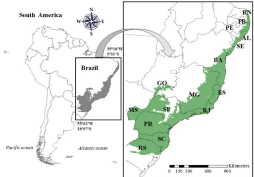
FIGURE 1 Original distribution of Brazilian Atlantic Forest hotspot (in gray) in South
864
America. Brazilian states: RS: Rio Grande do Sul; SC: Santa Catarina; PR: Paraná; 865
MS: Mato Grosso do Sul; SP: São Paulo; GO: Goiás; MG: Minas Gerais; RJ: Rio de 866
Janeiro; ES: Espirito Santo; BA: Bahia; SE: Sergipe; AL: Alagoas; PE: Pernambuco: 867
PB: Paraíba; RN: Rio Grande do Norte. 868
869 870 871