BJRS
RADIATION SCIENCES
07-02B (2019) 01-16ISSN: 2319-0612 Accepted: 2019-02-22
Simplified CFD model of coolant channels typical of a
plate-type fuel element: an exhaustive verification of the
simulations
J. G. Mantecón; M. M. Neto
Instituto de Pesquisas Energéticas e Nucleares, IPEN-CNEN/SP, 05508-000, São Paulo, SP, Brasil [email protected]
ABSTRACT
The use of parallel plate-type fuel assemblies is common in nuclear research reactors. One of the main problems of this fuel element configuration is the hydraulic instability of the plates caused by the high flow velocities. The current work is focused on the hydrodynamic characterization of coolant channels typical of a flat-plate fuel element, using a numeri-cal model developed with the commercial code ANSYS CFX. Numerinumeri-cal results are compared to accurate analytinumeri-cal solutions, considering two turbulence models and three different fluid meshes. For this study, the results demonstrated that the most suitable turbulence model is the k- model. The discretization error is estimated using the Grid Conver-gence Index method. Despite its simplicity, this model generates precise flow predictions.
1. INTRODUCTION
In nuclear research reactors, it is common the use of parallel plate-type fuel assemblies due to its high power density. To remove heat generated by fission reactions, the coolant flows over the plates with high velocity. One of the main problems of this fuel element configuration is the hydraulic instability of the plates caused by the high flow rate [1].
The analysis of the deflection of plate-type fuel due to high flow rate has taken place for many years. One of the first published reports regarding flow-induced deflections of this fuel element geometry was written by Stromquist and Sisman in 1948 [2]. The study was performed in a mockup and it was found that when the fluid velocity was raised to sufficiently high values, fuel plates de-formed plastically. In 1958 the same problem was detected by Ronald Doan in the Engineering Test Reactor (ETR). Doan discussed a critical flow field related to the plate deflection [3]. The Doan’s hypothesis was used by Miller, who provided a method for predicting the critical velocity based on the Bernoulli theory of incompressible flow. Miller’s analysis gave a basic idea of how the plates within a plate-type fuel assembly tend to deflect and a good approximation for that flow rate which induces a plate to deflect [1]. After Miller’s work, many researchers around the world have been studying this fuel assembly type. Earlier methods for assessing fuel plate deflection and coolant flow across channels have relied on analytical and experimental techniques [4]–[8]. The last years, although a continued development and cost-effectiveness of computational techniques has occurred, a limited number of works have been conducted applying the Computational Fluid Dynamics (CFD) technique for describing that fuel element configuration [9]–[11].
In CFD studies an accurate solution it is a combination of an effective selection of the grid size and, in the case of turbulent flows, an adequate choice of the turbulence model. The procedure for de-termining the most accurate mesh is to carry out simulations with different mesh sizes and configu-rations until the numerical solution converges, in what is named the grid convergence study. Two parameters need to be considered when a grid convergence study is executed: computation time and accuracy. Which a finer grid the solution tends to become more accurate, but the calculation time required for achieving it increases. Therefore, the purpose of a grid convergence study is to reach a reasonably precise solution without taking an excessive time. On the other hand, turbulent flows are
significantly affected by the presence of walls (e. g. flow across parallel-plate fuel assemblies) and a correct presentation of the near-wall region determines a successful prediction of wall-bounded tur-bulent flows. When dealing with turtur-bulent flows a good strategy for selecting the corresponding turbulence model is based on wall y+ value [12].
When CFD analyses are conducted, the verification of numerical solution is extremely important. According to Oberkampf and Roy [13], the “solution verification addresses the question of whether a given simulation of a mathematical model is sufficiently accurate for its intended use”. In other words, the computational results are compared with highly accurate benchmark solutions, usually analytical solutions. Additionally, as occurs in experiments, in numerical models there is an uncer-tainty associated. It is generally accepted that the numerical error of CFD calculation has three error components: the iterative error, the round-off error and the discretization error [14]. Procedures for numerical error estimation usually assume that the contribution of the round-off and iterative errors is negligible compared to the discretization error. A well-established method for error estimation caused by discretization is the Grid Convergence Index (GCI) method [15].
The current study is focused on the hydrodynamic characterization of coolant channels typical of a plate-type fuel element. For this purpose, mesh refinement tests are performed, considering three different meshes; also, two turbulence models are studied: k- and k-, with the commercial code ANSYS CFX [16]. For determining the CFD discretization error the GCI method is used and the numerical results are compared to precise analytical solutions. It is essential to highlight that this work helps to select the mesh and turbulence model that will be considered in an upcoming co m-plex research. In the near future, a series of simulations will be conducted to understand the fluid-structure interaction (FSI) phenomenon in a plate-type fuel element and this work is the first step.
2. METHODOLOGY
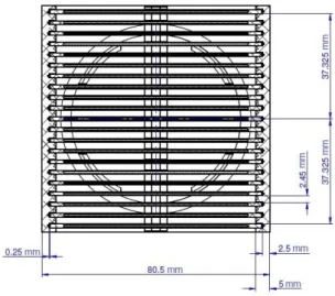
The model is developed considering the geometric data of the future Brazilian Multipurpose Reac-tor (RMB by its acronyms in Portuguese) fuel elements. Erro! Fonte de referência não
Figure 1: Cross-sectional view of the fuel element.
2.1. Near-Wall Treatment
In near-wall fluid flow, the flow gradient normal to the wall tends to develop on small scales. In that region, a fine mesh is needed to be able to capture the effects of the boundary layer. A parameter used to describe how fine or coarse is a mesh for a particular flow model is the wall y+. It is the ra-tio between the turbulent and laminar influences in a cell. Near wall-regions the viscosity-affected region is made up of three zones, with their corresponding wall y+ [17]:
▪ Viscous sublayer (y+ ≤ 5),
▪ Buffer layer or blending region (5 < y+ < 30),
▪ Fully turbulent region or log-law region (y+ ≥ 30 up to 100).
While directly solving for the near wall flow (y+ < 5) may provide a more precise solution, it also
requires very fine mesh in the near-wall zone and, correspondingly, higher computer-storage re-quirements and longer run times. In contrast, when high y+ wall treatment is used (y+ ≥ 30), the near
wall velocity distribution is assumed to follow the log-law and it is considered that the centroids of wall-bounding cells are within that region. This allows the use of coarse meshes near to the wall to resolve the velocity profile.
Typically are recommended values of y+ close to the lower bound (≈ 30) when wall functions are considered, whereas y+ ≈ 1 is more desirable for near-wall modeling [12]. Wall functions are the
turbulence models based on the -equation; for -based models the Automatic Near-Wall Treat-ment method is applied. In this work is a desire to resolve the boundary layer in the log-law region.
2.2. The Grid Convergence Index Method
In CFD studies, the analysis of the influence of mesh refinement in numerical solution is vital. In 2008 a “Procedure for estimation and reporting of uncertainty due to discretization in CFD applica-tions” was proposed by the Journal of Fluid Engineering editors [18]. This procedure consists in the estimation of the discretization uncertainty using the Grid Convergence Index method.
The GCI method was developed by Roache [15] and it is based on the Richardson Extrapolation, involving comparison of solutions at different grid spacing [19]. The GCI gives a prediction on how much the solution would change with a further refinement of the mesh. A small value of the GCI is preferred. For three-dimensional calculations, a representative grid size h is calculated using the following equation:
(1)
where Vi is the volume of the ith cell and N is the total number of cells. In this work, three
differ-ent grids were used (coarse - Mesh 3, medium - Mesh 2, and fine - Mesh 1) with the refinemdiffer-ent factor between grids r = hcoarse/hfine. The calculation of the apparent order of the method (p) can be
done using the expressions:
(2a)
(2b)
(2c) Being, ε32 = ϕ3 – ϕ2, ε21 = ϕ2 – ϕ1 and ϕ3, ϕ2, ϕ1 are the coarse-, medium- and fine grid solution of
the variable of interest obtained with the three grid sizes h3, h2 and h1, respectively. If r is constant
then q(p) = 0. The approximate relative error can be calculated as:
(3) Then, the GCI for the finest mesh is:
(4)
2.3. Numerical Model
To solve a fluid mechanics problem with CFD a basic practice must be followed. First, the geome-try of the fluid domain must be created. Second, the geomegeome-try is discretized into small volumes. Once the mesh is created, the correct physics model and boundary conditions must be chosen.
Figure 2: Fluid domain considering two coolant channels.
Erro! Fonte de referência não encontrada. shows a generic diagram of the fluid domain. This
geometry will be used in both numerical and analytical modeling. In the figure, the “Void Region” is the position where the fuel plate is located. In this case, that zone is considered empty because the plate is not modeled. The arrows on the top indicate de flow direction. Table 1Erro! Fonte de
refe-rência não encontrada. are listed the geometric parameters and water properties considered.
Ac-cording to the RMB project designers, the average fluid velocity (v) through the coolant channels is 8.2 m/s [20]. Then, at the inlet surface, the “velocity inlet” boundary condition was set using the Equation (5) to guarantee an average channel velocity close to the project. This equation was estab-lished considering the law of mass conservation and that the flow is incompressible.
Table 1: Geometric parameters and fluid properties.
Channel 1 thickness (a) 2.45 mm Channel 2 thickness (b) 2.45 mm Plate thickness (c) 1.35 mm Channels width (d) 70.5 mm Inlet length (Li) 190.0 mm Plate length (Lp) 655.0 mm Outlet length (Lo) 70.0 mm Density () 997.561 kg/m3
Dynamic viscosity () 8.871e-4 Pa∙s
The outlet boundary condition was set as a zero-pressure boundary. For the plate surfaces and the walls enclosing channels, no-slip smooth wall condition was chosen. The coolant channels were set with equal thicknesses so the CFD model could be easily benchmarked to a simple 1D analytical model. All simulations were run to steady state.
(5) To capture the contraction/expansion effects at the leading/trailing edges of the plate, a bias factor 4:1 was set up for spacing the cells along the inlet, outlet, and plate lengths, and for the cells through the thickness of the channels. The bias factor is defined as the ratio of the longest division and the shortest division. The geometry includes regions for flow development at the inlet and exit of the plate region. It was partitioned allowing the creation of structured meshes. Erro! Fonte de
referência não encontrada. 2 shows the number of cells in all directions.
Table 2: Number of elements in all directions. Mesh Li Lp Lo d a b c Total
1 (fine) 80 200 50 52 16 16 16 657280
2 (medium) 80 200 50 52 11 11 11 451880
The wall y+ value in the fluid solution will be dictated by the thicknesses of the wall-bounding cells. The establishment of the mesh depends on the choice of the grid refinement factor. Although usual-ly r = 2 is used, i.e. grid doubling (halving), this would lead to an increase of 23 of the number of volumes, resulting in an excessive computational time. According to Stern et al. [21], for CFD ap-plications a good alternative is to use r = 21/2. The fluid mesh is depicted in the next figure.
Figure 3: Coarse mesh – leading edge region.
Since the coolant flow through the fuel element is turbulent, a turbulence model must be utilized to generate precise flow predictions. Numerous turbulence models have been developed with the most popular being the Reynolds Averaged Navier-Stokes (RANS) variety. In this work, a study compar-ing turbulence models was completed takcompar-ing into consideration two RANS models: realizable k- and standard k-. These turbulence models have demonstrated to be very useful for simulating the flow through a duct [22].
Residual values of 1e-5 for the mass/momentum and turbulent transport equations are monitored during the simulations, usually sufficient for most engineering applications. Other important criteria to confirm the solution convergence is the net mass imbalances. The net mass imbalance to be deemed converged should be less than 0.1%. The energy equation is neglected.
2.4. Analytical Model
A simple analytical model to estimate the overall pressure drop through the geometry was employed for verification purpose. The pressure drop can be determined by taking into account the flow con-traction at the leading edge of the plate, flow expansion at the trailing edge, and frictional losses (see Erro! Fonte de referência não encontrada.):
(6) Pin, Pch, and Pout are the pressure drop caused by friction at the inlet plenum, coolant channel
region, and outlet plenum, respectively. PSC is due to the abrupt contraction and PSE because of
the sudden expansion. The terms of the equation before can be defined as:
(7a)
(7b)
(7c) where is the fluid density, Dh,i and Dh,o are the hydraulic diameters at inlet and outlet of the form
loss junction, respectively; Dh,in is the hydraulic diameter of the inlet and outlet plenum, and Dh,ch
the hydraulic diameter of the coolant channel. The Darcy friction factor (f) is solved using the Haa-land equation [17], considering smooth surfaces:
(8) Re is the Reynolds number in the region of interest. In addition to pressure drop, an analytical solu-tion for the wall shear stress (τ) is practical informasolu-tion for benchmarking. The following equasolu-tion is used to calculate the wall shear stress [17]:
3. RESULTS AND DISCUSSION
An exhaustive verification procedure was conducted for selecting a suitable combination of mesh and turbulence model. The criteria utilized to decide the most appropriate turbulence model is the accurateness of the pressure drop and the wall shear stress solutions when compared to an analytical solution. Once it selected, the GCI method is employed to find the uncertainty due to discretization. During simulations, the average y+ value on the plate surfaces parallel to fluid was monitored. As a
result of the grid refinement along channel thicknesses, a y+ value nearly 30 was reached. Table 3
details the average y+ value for each case.
Table 3: Average y+ value for each mesh and turbulence model.
Model y
+
Mesh 3 Mesh 2 Mesh 1
k- 51.75 51.73 33.21
k- 51.72 51.74 33.73
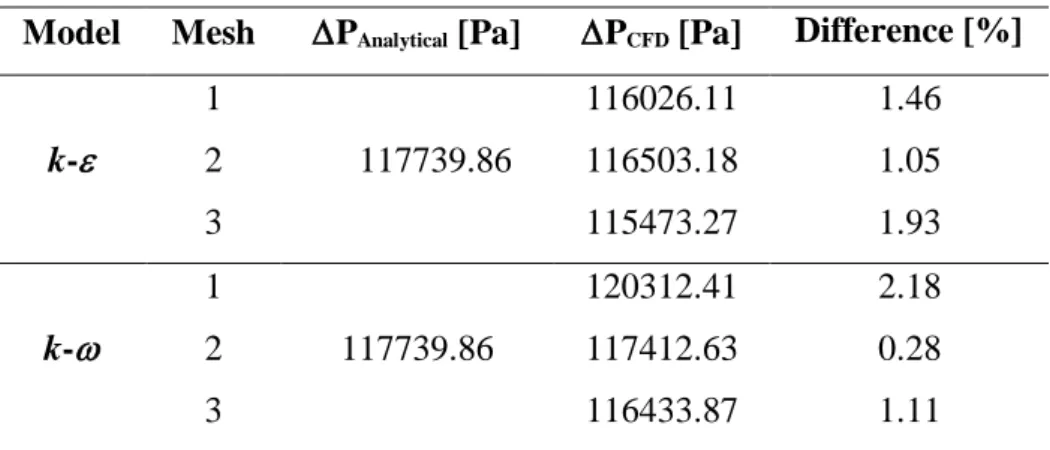
Erro! Fonte de referência não encontrada. shows the overall pressure drop through the geometry.
Table 4: Results of pressure drop.
Model Mesh PAnalytical [Pa] PCFD [Pa] Difference [%]
k- 1 117739.86 116026.11 1.46 2 116503.18 1.05 3 115473.27 1.93 k- 1 117739.86 120312.41 2.18 2 117412.63 0.28 3 116433.87 1.11
In Table 4 can be seen that the k- turbulence model with Mesh 2 has a better agreement with the analytical result but this configuration is not the proper one because y+ = 51.74. Besides, when the
number of cells increases from Mesh 2 to Mesh 1, the pressure drop difference also rise to 2.18%, considered a high value if it is compared to the k- model solutions. On the other hand, the pressure drop solution with k- model shows very good agreement with the analytical model; in all cases, the difference is less than 2.00%.
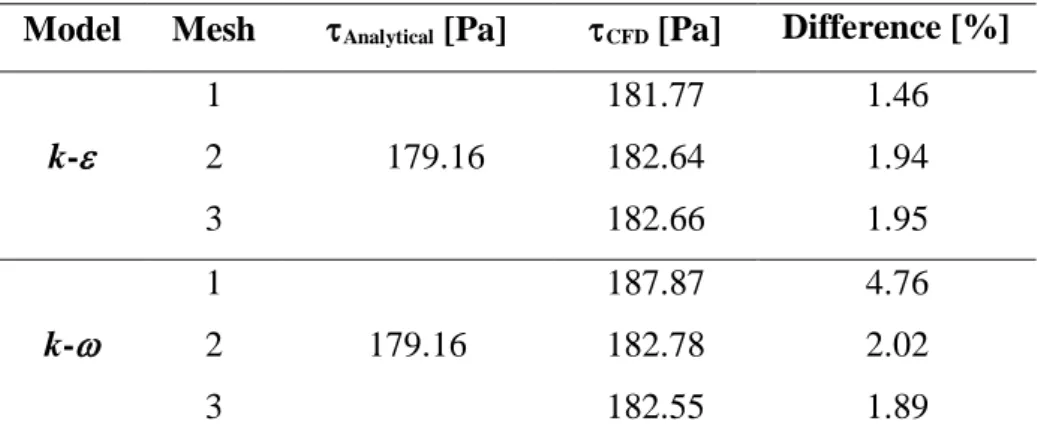
Table 5 shows the wall shear stress results. With k- model, the wall shear stress results move away from the analytical solution with the mesh refinement. However, using the k- formulation the pre-dictions are closest to the reference value in all three cases. The increment of the number of ele-ments leads to the difference reduction between the numerical and analytical model. The best result is achieved with Mesh 1 and the deviation from the analytical solution is only 1.46%.
Table 5: Results of wall shear stress.
Model Mesh Analytical [Pa] CFD [Pa] Difference [%]
k- 1 179.16 181.77 1.46 2 182.64 1.94 3 182.66 1.95 k- 1 179.16 187.87 4.76 2 182.78 2.02 3 182.55 1.89
Another parameter used to verify the numerical solution was the average fluid velocity in the cool-ant channels. Table 6 shows a comparison between the average velocity obtained with the CFD model and the velocity proposed by the RMB project designers. The difference was also estimated. As a result of the mesh improvement, the average fluid velocity is close to the design velocity. The best result is achieved taking into account the k- formulation with the fine mesh (difference of 0.12%). In Figure 4 pressure and velocity contour plots, located at the leading edge, are depicted. As it is expected, the maximum pressure is obtained at the leading edge and higher velocities along coolant channels.
Even though one specific variable can match better the analytical solution considering a particular mesh and turbulence model combination, generally k- model performs very well for the metrics
employed (pressure drop, wall shear stress, and average fluid velocity). From the results, it is clear that the k- model joint with Mesh 1 is the best option for matching the analytical solution. There-fore, for future FSI analysis, the model will use a fine mesh (Mesh 1) with the k- formulation.
Table 6: Results of average fluid velocity.
Model Mesh vProject [Pa] vCFD [Pa] Difference [%]
k- 1 8.2 8.19 0.12 2 8.18 0.24 3 8.12 0.95 k- 1 8.2 8.16 0.49 2 8.12 0.98 3 8.07 1.59
Figure 4: Contour plots of (a) pressure and (b) velocity at the leading edge region, using
the k- model and Mesh 1.
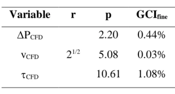
With the previous results and the methodology described in Section 2.2, the Grid Convergence In-dex was estimated. The GCI calculation for the selected variables is shown in Table 7. It can be
observed that the numerical uncertainty of the fine-grid solution is less than 1.10% for all cases. Thus, the discretization is accurate and further mesh refinement is not essential.
Table 7: GCI calculations. Variable r p GCIfine
PCFD 21/2 2.20 0.44% vCFD 5.08 0.03% CFD 10.61 1.08%
4. CONCLUSION
In this work, a numerical model for the hydrodynamic characterization of coolant channels typical of a parallel-plate fuel assembly was presented. To achieve precise results, two turbulence models were explored considering three different fluid meshes. For selecting a suitable combination of tur-bulence model and mesh, the results of pressure drop and wall shear stress were compared to accu-rate analytical solutions. Wall y+ was used to decide which mesh and turbulence model are the most
appropriates. In some cases using the k- model better predictions were achieved, but the mesh and turbulence model combination was not the adequate because of the wall y+ value. Results
demon-strated that the k- model match with high precision the analytical solutions. In all cases, the devia-tion from the analytical soludevia-tions was less than 2%. The model produced results consistent with the theory. In particular, the maximum pressure was noticed at the leading edge and higher velocities along channels.
In addition, as part of solution verification procedure of the numerical model, the uncertainty due to geometry discretization was calculated. For this purpose, the GCI of the variables of interest was evaluated. For the three variables selected, the GCI was less than 1.10%, demonstrating that the discretization is accurate and additional mesh refinement is not required. The GCI concept is an objective and very comprehensive procedure for discretization error estimation. Considering the results of this work, it is clear that k- model with Mesh 1 is a very good mesh/turbulence model combination for the fluid-structure interaction analysis.
5. ACKNOWLEDGMENT
The authors are grateful to CAPES foundation for the financial support.
REFERENCES
[1] MILLER, D. R. Critical flow velocities for collapse of reactor parallel-plate fuel assemblies. J.
Eng. Power, v. 82, p. 83–91, 1960.
[2] STROMQUIST, W. K.; SISMAN, O. High Flux Reactor fuel assemblies vibration and water
flow. ORNL-50, Oak Ridge, 1948, 55p.
[3] DOAN, R. L. The engineering test reactor - a status report. Nucleonics, v. 16, 1958.
[4] SMISSAERT, G. E. Static and dynamic hydroelastic instabilities in MTR-type fuel elements Part I. Introduction and experimental investigation. Nucl. Eng. Des., v. 7, p. 535–546, 1968.
[5] SMISSAERT, G. E. Static and dynamic hydroelastic instabilities in MTR-type fuel elements Part II. Theoretical investigation and discussion. Nucl. Eng. Des., v. 9, p. 105–122, 1969.
[6] GUO, C. Q.; PAIDOUSSIS, M. P. Stability of Rectangular Plates with Free Side-Edges in Two-Dimensional Inviscid Channel Flow. J. Appl. Mech., v. 67, p. 171–176, 2000.
[7] LI, Y.; LU, D.; ZHANG, P.; LIU, L. Experimental investigation on fluid-structure interaction phenomenon caused by the flow through double-plate structure in a narrow channel. Nucl. Eng.
Des., v. 248, p. 66–71, 2012.
[8] HOWARD, T. K.; MARCUM, W. R.; JONES, W. F. A novel approach to modeling plate de-formations in fluid-structure interactions. Nucl. Eng. Des., v. 293, p. 1–15, 2015.
[9] CURTIS, F. G.; EKICI, K.; FREELS, J. D. Fluid-Structure Interaction for coolant flow in re-search-type nuclear reactors, In: COMSOL CONFERENCE, 2011, Boston, 2011.
[10] KENNEDY, J. C.; SOLBREKKEN, G. L. Coupled Fluid Structure Interaction (FSI) modeling of parallel plate assemblies, In: PROCEEDINGS OF THE ASME 2011 INTERNATIONAL
MECHANICAL ENGINEERING CONGRESS & EXPOSITION, 2011, Denver: American
Society of Mechanical Engineers, 2011.
[11] BODEY, I. T.; CURTIS, F. G.; TRAVIS, A. R., ARIMILLI, R. V; FREELS, J. D. Research
and development of multiphysics models in support of the conversion of the High Flux Isotope Reactor to low enriched uranium fuel. ORNL/TM-2015/656, Oak Ridge, 2015, 227p.
[12] SALIM, S. M.; CHEAH, S. C. Wall y+ strategy for dealing with wall-bounded turbulent flows,
In: PROCEEDINGS OF THE INTERNATIONAL MULTICONFERENCE OF ENGINEERS
AND COMPUTER SCIENTISTS, 2009, Hong Kong, 2009. p. 1–6.
[13] OBERKAMPF, W. L.; ROY, C. J. Verification and validation in scientific computing. New York: Cambridge University Press, 2010.
[14] EÇA, L.; HOEKSTRA, M. A procedure for the estimation of the numerical uncertainty of CFD calculations based on grid refinement studies. J. Comput. Phys., v. 262, p. 104–130, 2014.
[15] ROACHE, P. J. Verification and validation in computational science and engineering. Al-buquerque: Hermosa Publishers, 1998.
[16] ANSYS Inc. ANSYS CFX Documentation, Release 18. Canonsburg, 2016.
[18] CELIK, I. B.; GHIA, U.; ROACHE, P. J.; FREITAS, C. J.; COLEMAN, H.; RAAD, P. E. Pro-cedure for estimation and reporting of uncertainty due to discretization in CFD applications. J.
Flu-ids Eng., v. 130, p. 1–4, 2008.
[19] RICHARDSON, L. F. The approximate arithmetical solution by finite differences of physical problems involving differential equations, with an application to the stresses in a masonry dam.
Philos. Trans. R. Soc. A, v. 210, p. 307–357, 1911.
[20] INVAP, Brazilian Multipurpose Reactor project - core thermal-hydraulic design in
forced convection, RMBP-0130-2IIIN-005-A, 2013, 18p.
[21] STERN, F.; WILSON, R. V.; COLEMAN, H. W.; PATERSON, E. G. Comprehensive ap-proach to verification and validation of CFD simulations - Part 1: methodology and procedures. J.
Fluids Eng., v. 123, p. 793–802, 2001.
[22] ANDERSON, J. D.; DEGROOTE, J.; DEGREZ, G.; DICK, E.; GRUNDMANN, R.;VIERENDEELS, J. Computational Fluid Dynamics: An Introduction, 3rd ed. Berlin: Spring-er, 2009.