M
ASTER
ACTUARIAL SCIENCE
M
ASTER
´
S
F
INAL
W
ORK
DISSERTATION
M
ORTALITY OF
E
LITE
A
THLETES
:
A
N
A
PPLICATION TO
F
OOTBALL
P
LAYERS
INÊS
FILIPA
COSTA
MARQUES
M
ASTER
ACTUARIAL SCIENCE
M
ASTER
´
S
F
INAL
W
ORK
DISSERTATION
M
ORTALITY OF
E
LITE
A
THLETES
:
A
N
A
PPLICATION TO
F
OOTBALL
P
LAYERS
INÊS
FILIPA
COSTA
MARQUES
S
UPERVISION
:
ONOFRE
ALVES
SIMÕES
Abstract
The health benefits of moderate regular physical activity have been clearly demonstrated and are widely consensual. However, there is a growing debate over the potential adverse effects of strenuous physical activity, particularly at a professional level. Recent findings of cardiovascular anomalies in elite athletes coupled with the high frequency of injuries have brought some sports under increased scrutiny.
In this context, the main goal of this work is to investigate whether elite athletes live longer than the general population. After an initial review of the literature on elite athletes’ mortality, a comprehensive survival analysis is applied to two populations of professional football players.
Lifespan data and specific occupational variables of Portuguese and Spanish football players, who have represented their national teams in their career, were collected from recognized publicly available sources. Each cohort is then compared to the respective standard population, using available data in the Human Mortality Database, through the estimation of standardised mortality ratios and survival curves. The years-lost method is applied to provide a time dimension measure for these elite athletes’ longevity. Furthermore, the association of position on the field and the number of games with overall mortality is accessed using Cox Proportional Hazard Models. At the end, a comparison between the mortality of Portuguese and Spanish football players is carried out.
Keywords: elite athletes, mortality, longevity, standardised mortality ratio, survival curve, years-lost method, Cox Proportional Hazard Models
Resumo
Os benefícios para a saúde resultantes da prática regular de exercício físico, de uma forma moderada, estão cientificamente comprovados. Contudo, quando se trata de uma abordagem sobre atletas profissionais, cuja actividade física é muito intensa, os benefícios deixam de ser uma clara evidência, surgindo por vezes sinais de alerta para os seus possíveis efeitos adversos. Para alimentar esta controvérsia, muito têm contribuído os estudos recentes que evidenciam anomalias e doenças cardiovasculares, bem como as frequentes lesões em atletas de elite.
É neste contexto que surge o principal objectivo deste trabalho: investigar se os atletas de elite vivem mais do que a população em geral. Após uma profunda revisão literária inicial relativa à mortalidade dos atletas de elite, procede-se a uma análise de sobrevivência que tem como foco dois grupos de jogadores de futebol profissionais.
Recolheram-se dados relativos à data de nascimento e morte (se for o caso) dos jogadores portugueses e espanhóis que representaram a sua selecção, bem como de outras variáveis de interesse para o estudo. Cada grupo de jogadores é comparado com a população geral do respectivo país, usando dados disponíveis na Human Mortality Database, através da estimação de standardised mortality ratios e de curvas de sobrevivência. O years-lost method é também aplicado, fornecendo uma medida de longevidade dos referidos atletas de elite. Ainda é averiguado se a posição dos jogadores e o número de jogos na sua carreira afectam diferencialmente a mortalidade dos mesmos, através dos Cox Proportional Hazard Models. Por fim, as populações dos jogadores portugueses e espanhóis são comparadas entre si.
Palavras-chave: atletas de elite, mortalidade, longevidade, standardised mortality ratio, curva de sobrevivência, years-lost method, Cox Proportional Hazard Models
Acknowledgements
I would like to start by thanking my supervisor, Professor Onofre Alves Simões, for his indispensable support, valuable suggestions and availability. I am particularly grateful for not letting me quit the subject of the thesis when I thought I did not have sufficient information to proceed.
I extend my profound appreciation to Professor Eduardo Trigo for providing sources of data for the study.
I am also thankful to all Professors of the Master’s Degree for their insightful lectures and patience for my endless questions.
I also express my gratitude to Tranquilidade for the opportunity of doing an internship, allowing the development of my actuarial skills. The attendance of the R software course was particularly helpful in the progress of the thesis. I would like to thank my colleagues of the Non-Life Actuary Department for making me feel part of the team since the beginning.
The warmest thanks go to my family. To my parents, who have equipped me with all the tools and skills to be successful in any career path I decided to follow. To my grandmother, who provided me the best place to work and the most delightful breaks. I wish you were here to celebrate one more accomplishment. To my brother for not letting me down with his good humor during the periods of low energy and motivation. To João, for the unconditional support, generosity, understanding and for always believing in me. I am fortunate to have you in my life.
Table of contents
Abstract... iii
Resumo ... iv
Acknowledgements ...v
List of Abbreviations ... viii
List of Figures... ix
List of Tables ...x
Chapter 1 – Introduction ...1
Chapter 2 – Literature Review ...4
Chapter 3 – Methods to quantify and compare mortality ...8
3.1 Measures of comparative mortality ...8
3.1.1 General notation ...9
3.1.2 Computation of central exposed to risk ...9
3.1.3 Crude Mortality Rate (CMR) ...12
3.1.4 Directly Standardised Mortality Rate (DSMR) ...13
3.1.5 Indirectly Standardised Mortality Rate (ISMR) ...13
3.1.6 Standardised Mortality Ratio (SMR) ...14
3.2 Observed and expected survival function ...16
3.2.1 Kaplan-Meier method – Estimation of observed survival ...16
3.2.2 Estimation of expected survival ...17
3.3 Years of Life Lost/Saved ...20
3.4 Cox Proportional Hazard Models ...22
Chapter 4 – Applications ...24
4.1 Mortality of Portuguese Football Players ...25
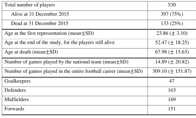
4.1.1 Data collection and statistical analysis ...25
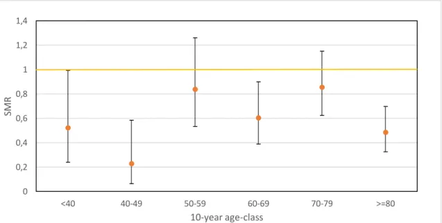
4.1.2 Results ...26
4.2 Mortality of Spanish Football Players ...31
4.2.1 Data collection and statistical analysis ...31
4.2.2 Results ...32
4.3 Comparing the mortality of Portuguese and Spanish football players ...38
Chapter 5 – Conclusion ...40
Appendix ...43
A. Hypothesis test for the standardised mortality ratio...43
C. SMR and 95% CI for every setting of age/time-periods ...45
D. Cox Proportional Hazard Models ...46
References ...47
viii
List of Abbreviations
Abbreviation Meaning
ALS Amyotrophic Lateral Sclerosis BMI Body Mass Index
CI Confidence Interval HMD Human Mortality Database
HR Hazard Rate
NFL National Football League SMR Standardised Mortality Ratio US United States
ix
List of Figures
3.1–Lexis diagram divided into 1x1 cells (one year of age by one year of time) to illustrate
the follow-up of a hypothetic individual and the computation of his exposure to risk ……....11
4.1–SMR for Portuguese football players by 10-year age class and respective 95% CI ...27
4.2–Portuguese football players observed and expected survival curves………....28
4.3–SMR for Spanish football players by 10-year age class and respective 95% CI ...34
4.4–Spanish football players observed and expected survival curves………...35
x
List of Tables
3.1–Central exposed to risk (in days) by age and calendar year for the hypothetic individual...11 3.2–Example of computation of CMR to illustrate that this measure can be misleading if used to compare the two populations. Adapted from: IFOA (2011), Core Reading: Subject CT5,
Chapter 15………...12
3.3–Illustration of age and calendar year specific annual survival probabilities……….18 4.1–Characteristics of Portuguese Football Players (1921-2015 period). Sources: FPF;
Zerozero.pt; national-football-teams and eu-football.info……….…....26
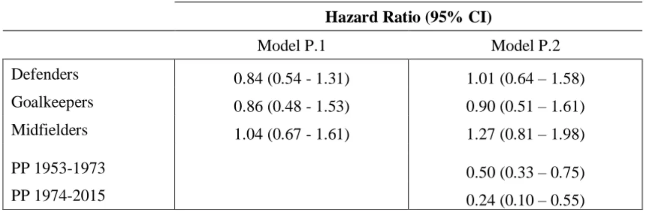
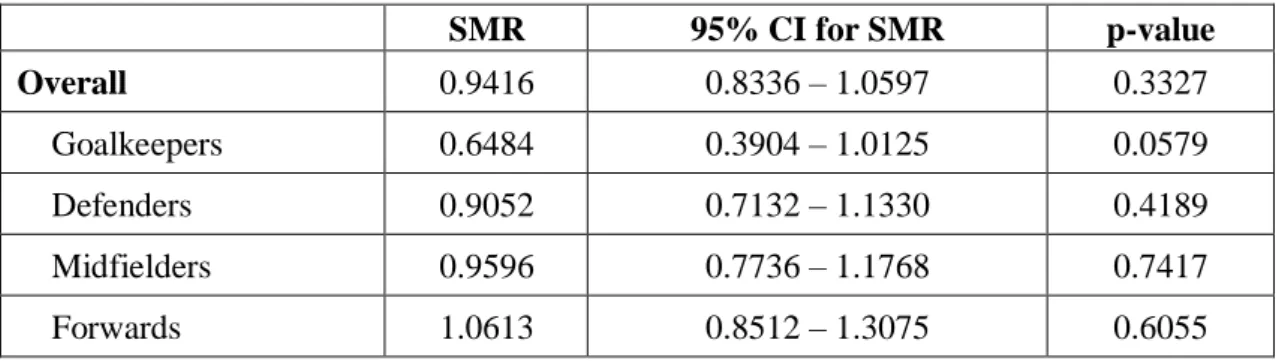
4.2–SMR for Portuguese football players, 95% CI and p-value: overall and stratified by position...27 4.3–Standardised mortality ratio over time (four periods) for Portuguese football players…28 4.4–Cox proportional hazard ratios and 95% CI for number of games (model G.1 – adjusted for age; model G.2 – adjusted for age and period of participation) for Portuguese football players...30 4.5–Cox proportional hazard ratios and 95% CI for position on the field (model P.1 – adjusted for age; model P.2 – adjusted for age and period of participation) for Portuguese football players………30 4.6–Cox proportional hazard ratios and 95% CI for multivariate models including number of games and position on the field (model GP.1 – adjusted for age; model GP.2 – adjusted for age and period of participation) for Portuguese football players………...30 4.7–Characteristics of Spanish Football Players (1920-2014 period). Sources: AEDFI; Bdfutbol; national-football-teams and eu-football.info……….32
4.8–SMR for Spanish football players, 95% CI and p-value: overall and stratified by position...33 4.9–Standardised mortality ratio over time (five periods) for Spanish football players…....34
xi
4.10–Cox proportional hazard ratios and 95% CI for number of games (model G.3 – adjusted for age; model G.4 – adjusted for age and year of birth) for Spanish football players…....….36 4.11–Cox proportional hazard ratios and 95% CI for position on the field (model P.3–adjusted for age; model P.4 – adjusted for age and year of birth) for Spanish football players……...36 4.12–Cox proportional hazard ratios and 95% CI for multivariate models including number of games and position on the field (model GP.3 – adjusted for age; model GP.4 – adjusted for age and year of birth) for Spanish football players………...37 4.13–Single figure measures of mortality (CMR, DSMR and ISMR) for Spanish and Portuguese football players based on two different standard populations………...38 C.1–SMR, 95% CI and p-value for Portuguese football players...45 C.2–SMR, 95% CI and p-value for Spanish football players...45 D.1–Cox proportional hazard ratios and 95% CI, using follow up as time scale, for Portuguese football players (model 1 – HR for number of games, adjusted for period of participation; model 2 – HR for position on the field, adjusted for period of participation; model 3 – HR for number of games and position on the field, adjusted for period of participation) ...46 D.2–Cox proportional hazard ratios and 95% CI, using follow up as time scale, for Spanish football players (model 1 – HR for number of games, adjusted for age at first match and year of birth; model 2 – HR for position on the field, adjusted for age at first match and year of birth; model 3 – HR for number of games and position on the field, adjusted for age at first match and year of birth)...46
1
Chapter 1 – Introduction
Nowadays, there is little doubt that regular physical exercise is beneficial for the individuals’ well-being, contributing to the prevention of cardiovascular diseases, hypertension, obesity, depression and some types of cancer, such as colon, breast, and lung (Hurley and Reuter, 2011). The World Health Organization (WHO, 2010) recommends that children should spend at least 60 minutes of moderate to vigorous-intensity physical activity daily, while adults are advised to do at least 150 minutes throughout the week. For additional health benefits, people are encouraged to increase these durations and to incorporate muscle-strengthening activities. In a study about the association between the different intensities of physical exercise and longevity, using a cohort of 13 485 men who have enrolled as undergraduates in Harvard University in the period 1916-1950, the authors conclude that greater energy expenditure is associated with lower mortality and this trend is more pronounced for vigorous activities than for moderate activities (Lee and Paffenbarger, 2000).
However, recent controversy exists regarding the potential adverse effects of repeated exposure to high levels of physical exercise, such as those required at a professional sports level.
One of the topics of current debate is the increased susceptibility of elite athletes to cardiovascular diseases. High-competitive sports may lead to physiological changes in the heart: the cardiac chambers enlarge and the heart muscle becomes thicker than normal, which is usually known as “athlete’s heart”. It has been hypothesized that prolonged aerobic exercise is more prone to lead to these changes; therefore, groups of ultra-endurance athletes (including cyclists, Ironman triathlon athletes and ultra-marathon runners) have often been assessed to study this relationship. These unique athletes compete in events that can last up to 30 hours; they usually train between 20-40 hours per week and expend over 70,000 KJ/ week. In addition, it should be noted that the number of individuals participating in these events is continually increasing as evidenced by the number of new races established each year.
The results of the studies are somewhat conflicting. Some authors reach the conclusion that ultra-endurance exercise elevates oxidative stress, leading to the development of acute cardiac dysfunction as evidenced by electrocardiography abnormalities, myocardial injury or atherosclerosis, consequently increasing the risk of cardiovascular diseases and mortality (Knez, Coombes and Jenkins, 2006; Laslett, Eisenbud and Lind, 1996). La Gerche
2
affects the right ventricular, which correlates with increases in biomarkers of myocardial injury and it is more prevalent in athletes with a longer history of competitive sport. In contrast, other studies do not find measurable persistent abnormalities of cardiac function in ultra-endurance elite athletes, suggesting that the response to oxidative stress might be mitigated as a result of exercise-induced adaptations, such as increased antioxidant defense and less reactive oxygen species production (La Gerche et al., 2004).
In a comprehensive study assessing world-class endurance athletes (Pelliccia et al., 2010), no cardiovascular events occurred and uninterrupted training/competition over long periods of time (for more than eight years on average) was not associated with deterioration in left ventricular function, significant changes in left ventricular morphology or onset of symptoms of cardiomyopathies.
The debate on the consequences of heart remodeling in elite athletes and the safety of long-term and intense sports participation is fueled by news media reports of sudden cardiac deaths. The most shocking case in Portugal was the death of the professional football player Miklós Fehér at age 24, during a match (2004). The cause of death was cardiac arrhythmia, brought on by hypertrophic cardiomyopathy, which is known as a leading cause for cardiac arrests in young athletes and it usually asymptomatic.
Along with the premature deaths, the high frequency of injuries has brought some sports under increased scrutiny, especially those with a high risk of bodily collision and high physical contact. For instance, chronic traumatic encephalopathy is a progressive degenerative disease, most commonly found in elite athletes participating in American football, boxing, ice hockey and rugby, with a history of repetitive brain injuries, including symptomatic concussions (Koning et al., 2014; McKee et al., 2009; Zwiers et al., 2012). This disease leads to early onset dementia and it is associated with reduced life expectancy.
A number of studies have thus attempted to study the risk-benefit ratio of intensive exercise by assessing mortality in elite athletes. The scientific literature, which is reviewed in Chapter 2, provides a major evidence of lower mortality in elite athletes, as well as a higher life expectancy.
Following the brief introduction and the literature review, Chapter 3 introduces the main methods used to assess mortality of a population, with particular evidence given to its comparison to a standard population.
The main findings in the literature on elite athletes’ mortality vary according to nationality and sport practiced. In addition, the methods employed, the period of enrollment
3
in sports or the follow-up time provide large variations in the results. Consequently, estimates from these studies are not easily transposable to other elite populations.
An exhaustive research on this topic was performed and, to date, it was not found any study on the mortality/longevity of Portuguese athletes, whether among professional or amateurs, male or female. Given the interest in this population, the next step of this work involved the collection and creation of the data set, which revealed to be one of the most time-consuming tasks. It has implied contacting and visiting the Portuguese Federations of several sports, the Portuguese Institute of Sports and Youth (Instituto Português do Desporto e Juventude) and the office of the insurance company Fidelidade (which works with sports and health insurance of high performance athletes). At the end, internet has showed to be the best source of data. The only successful group of Portuguese elite athletes for whom it was possible to create a data set was the football players, in particular, those who have already represented the National Team. In order to have a broader study, data on Spanish football team players was also collected, resulting in an Iberian analysis.
The process of data collection, the statistical analysis and the results obtained are presented in Chapter 4, the main contribution of this paper. Regarding the software employed in this work, Excel was used for data set building and making simple analyses; R was the chosen tool to compute mortality measures and to develop regression models.
Finally, Chapter 5 includes the relevant conclusions, limitations of the study and topics for future research.
4
Chapter 2 – Literature Review
A majority of studies assessing elite athletes’ mortality and longevity shows that elite athletes survive longer than the general population, with these differences being more pronounced for endurance and mixed-sport athletes.
In two different studies of cyclists who have participated in the Tour de France, it was reported a substantially and significantly lower mortality in cyclists, compared to the general male population (Marijon et al., 2013; Sanchis-Gomar et al., 2011). These professional cyclists constitute one population of particular interest, since Tour de France is one of the most demanding and difficult sports event in the world, during which cyclists cover around 3500km in three weeks.
Sanchis-Gomar et al. (2011) consider the participants in the Tour de France between the years 1930 and 1964, excluding cyclists for whom they do not have proof of date of birth or death, who did not complete all stages and who were born in countries that have contributed with less than 100 participants during this period. The final sample consists of 834 cyclists, from France (n=465), Italy (n=196) and Belgium (n=173). Portuguese cyclists are not included, since they only represented 0.24% of the total number of participants. The authors compute the “percentage of survivors” for each age, given by the number of cyclists born in a given year who were alive on 31 December 2007, divided by the number of cyclists born in that given year. This survival rates are compared with those of the pooled general population of France, Italy and Belgium, for the appropriate birth cohorts (men born between 1892 and 1942, the years in which the cyclists studied were born). A polynomial regression curve of second order (Ribeiro, 2014; Wooldridge, 2012), in the age–survival (%) axis, is adjusted for each population and a non-parametric Mann-Whitney U test (Mann and Whitney, 1947) is applied for comparing the mean of the percent survival. The curve of the cyclists lies above the curve of the general population for all ages and by comparing the areas under the curves, the authors reach the conclusion that longevity of the cyclists is significantly higher (p<0.05). The estimated average of survival between 65 and 115 years is 39.1% in cyclists, while for the general population it is 21.5%. The authors also compare the age at which 50% of the population dies: 73.5 years for the general population vs. 81.5 years in the Tour de France participants.
In the study including only the French cyclists participating at least once in Tour de France from 1947 to 2012 (Marijon et al., 2013), the reduced mortality was confirmed with the calculation of standardized mortality ratios and their 95% confidence intervals, by
age-5
categories, calendar periods and specific causes of death, besides the overall ratio. A measure of longevity was also used, namely, the additional life span of cyclists who participated in the Tour between 1947 and 1951, which is estimated by 6.3 years compared to the reference population.
Lin, Gajewski, and Poznańska (2016) applied a parametric frailty survival model to a group of Polish athletes who have participated in the Olympic Games from 1924 to 2010. The study was restricted to the athletes born between 1890 and 1959, after concerns about medical improvements and the statistical power for parametric survival analysis. The authors fitted a ϒ-Gompertz hazard function to account for possible unobserved heterogeneity (ϒ; variance), which can arise from different region of birth, energy expenditure, nutrition and so on. The hazard function is given by 𝜇(𝑥) = 𝑎. 𝑒𝑏𝑥, therefore, the parameter b measures the rate of
ageing and a represents the magnitude of the hazard. The athletes were preassigned to two birth cohorts, 1890-1919 (cohort I) and 1920-1959 (cohort II), in order to account for socioeconomic changes and medical advancements. Results from cohort I suggest that Polish elite athletes exhibit lower risk of mortality and a slower rate of ageing (boly=0.08616) than
the general population from the same birth cohort (bhmd=0.09762). Regarding cohort II,
mortality risk is also lower for athletes than for the general population, however, the estimated rate of ageing is similar (boly=0.08467 and bhmd=0.08327). This last result may be attributed
to mortality improvements in Poland from year 1920 onwards. Actually, athletes benefited from a 50% reduction in mortality from cohort I to cohort II and the estimated overall mortality risk of the Polish general population is 29% lower in Cohort II than in I.
Sarna et al. (1993) estimated that Finnish long-distance runners and cross-country skiers, competing internationally between 1920 and 1965, live 5.7 years longer than age and area of residence-matched reference male cohorts in Finland.
Regarding team sports athletes, for example, baseball players (Abel and Kruger, 2005; Kalist and Peng, 2007) and National Football League (NFL) players (Koning et al., 2014) show lower mortality rates than general population.
There are many possible explanations for this apparent survival advantage of elite athletes. High physical fitness levels, achieved by daily vigorous exercise, are one of the crucial beneficial factors. Such excellence in sport is attained only by the healthiest and the fittest individuals, which may be partially explained by genetic predisposing factors; therefore, professional athletes are usually regarded as a select group. Moreover, elite athletes have a better access to quality health care, due to their medical team support and higher incomes in general. Commonly, they are no-smokers, follow a healthy diet and consume less
6
alcohol than the general population. Finally, elite athletes, especially endurance ones, tend to maintain these healthy lifestyle habits and remain active after retirement.
However, a few studies do not find a survival benefit of elite athletes. For example, Italian soccer players active in the three top leagues, between 1960 and 1996, do not show a mortality difference from the Italian population (Belli and Vanacore, 2005). Likewise, New Zealand rugby players had the same life expectancy as the general population (Beaglehole and Stewart, 1983).
Furthermore, there is a report by Pärssinen et al. (2000) observing that 12.9% of Finnish powerlifters died prematurely (mean age of death=43 years) compared to 3.1% of the general population during a 12-year follow-up period. The use of anabolic steroids to enhance performance and the higher prevalence of obesity and diabetes later in life are reasons proposed for the higher mortality of powerlifter athletes.
In some cases, an excess mortality by specific causes of death is observed for elite athletes, in comparison with standard population.
Two distinct studies conclude that Italian soccer players have considerably high death rates for diseases of the nervous system, mainly from amyotrophic lateral sclerosis (ALS). Belli and Vanacore (2005) reached a standardised proportionate mortality ratio for ALS of 11.58, when analysing Italian soccer players active in the period 1960-1996. Taioli (2007) studied a cohort of soccer players who were enrolled in the Italian A and B professional leagues for at least one season, between 1975 and 2003, recording a standardised mortality ratio for ALS of 18.18, without significant variation across calendar year.
Although the overall mortality was significantly reduced in the cohort of 3439 NFL players, with at least 5 pension-credited playing seasons from 1959 to 1988 (SMR=0.53), neurodegenerative mortality was estimated to be three times greater than that of the general US population, possibly related to the higher chronic traumatic encephalopathy (Lehman et
al., 2012).
In contrast to the studies presented before, where elite athletes are compared to the general population, in one article by Zwiers et al. (2012), the comparison is made among the Olympic athletes practicing sports with different levels of physical intensity and contact. The study assesses the mortality risk of 9889 athletes who participated in the Olympic Games between 1896 and 1936 in 43 different disciplines, which are classified in categories of: static intensity, dynamic intensity, cardiovascular intensity, physical contact and bodily collision. The authors calculate hazard ratios for all-cause mortality by using a left truncated Cox Proportional Hazard model (Cox, 1972). The results show that Olympic athletes engaging in
7
disciplines with increasing cardiovascular intensity are not associated with a significantly higher mortality risk. A separate analysis of the static and dynamic components shows similar non-significant results. These conclusions do not change under a multivariate analysis. The study points a higher mortality for those practicing sports with a high risk of bodily collision and high physical contact (hazard ratios of 1.11 and 1.16, respectively). A note for the fact that bodily collision becomes non-significant in a multivariate analysis, as a consequence of its close relation with physical contact. Identical analysis is developed for subgroups – men only, deaths after age 50, born before/after 1900 – and the results are similar to the mentioned above.
Other works show that mortality results vary even for athletes practicing the same sport. For instance, in the study including NFL players from two different seasons (Koning
et al., 2014), besides the analysis of overall mortality, the players are divided in subgroups,
by race, position played (line, skill and other) and number of games during their career. A Cox Proportional Hazard Model is developed to examine if the observable risk factors mentioned above influence mortality within the population of NFL players. There is evidence that line players have higher mortality than other players, which is expected since they are more susceptible to some kind of diseases (e.g.: cardiovascular diseases due to their higher body mass index (BMI)). In the 1970 cohort, white players exhibit a 33% lower hazard rate than non-white players, but this difference is no longer valid for the 1994 cohort. An interesting finding is that players who play more than two seasons worth of games face higher mortality rates than other players, registering a 347% higher hazard rate. In another study using a different cohort of NFL players, Baron et al. (2012) evaluated the association of position category and BMI with cardiovascular disease mortality. The BMI was treated as a categorical variable, with three levels: normal (18.5 to <25 kg/m2), overweight (≥25 to 30 kg/m2) and obese (≥30 kg/m2). Among other results, the authors found that CVD mortality was increased for players with BMI≥30kg/m2
in comparison to normal BMI (HR: 2.02; 95% CI: 1.06 – 3.85) and for defensive linemen compared to offensive linemen (HR: 2.07; 95% CI: 1.24 – 3.46).
8
Chapter 3 – Methods to quantify and compare
mortality
This chapter introduces the methodologies used to quantify and compare the mortality experience of different populations, and to monitor the progress over time of the populations’ mortality. In this analysis, there is a special focus on comparing the mortality of the population under study (specific cohort of elite athletes) with a standard population (reference/general population).
3.1 Measures of comparative mortality
One of the possible approaches involves the computation of summary (single figure) mortality indices. The general notation and definitions will be presented, having as main references the Core Reading - Subject CT5 in IFOA (2011), and Breslow and Day (1987).
In the context of comparing the mortality results of different populations, a problem arises if they have different structures with respect to background characteristics. One example is comparing mortality figures of populations (for example, Portuguese cyclists and Portuguese football players) with different age distributions. In this case, rates and ratios must be adjusted to ensure the comparability between the heterogeneous populations, a process known as standardisation, which has been used in actuarial applications since the mid-18th century (Keiding, 1987). Besides the example of age, mortality rates are commonly standardised by sex, race and calendar period. Other factors such as occupation, nutrition, housing, education and genetics, also contribute to differences in mortality (distorting variables); nevertheless, extensive data may be required so these adjustments are less frequently applied. Each population is said to be decomposed in groups (strata), having certain characteristics in common. Throughout this study, mortality rates are standardised by sex, age and calendar period. For example, one possible stratum could be: men, aged 30-35, during calendar period 1950-1955.
Mortality rates can be calculated either for total deaths or for separate causes of interest. However, only overall mortality rates are computed here, since it was not possible to obtain the cause of death for most athletes.
9
3.1.1 General notation
Considering that the population being studied is divided in 𝑀 classes (groups, strata), the following notation will be used for the cohort:
• 𝐸𝑗: central exposed to risk in class 𝑗 (𝑗 = 1, … , 𝑀) • 𝑑𝑗: number of deaths in class 𝑗 (𝑗 = 1, … , 𝑀) • 𝑚𝑗: central rate of mortality in class 𝑗 (𝑗 = 1, … , 𝑀)
The notation is modified by the addition of the superscript “𝑠” when it refers to the standard population, instead of the population under study. For example, 𝑆𝐸𝑗 is the central
exposed to risk in class 𝑗 in the standard population.
The central rate of mortality is preferentially used in population studies, in opposition to the initial rate of mortality (probability of death), 𝑞𝑥. This last one is obtained dividing the number of deaths, 𝑑𝑥, by the number of individuals alive at age 𝑥, 𝑙𝑥. Intrinsically, it is
assumed that 𝑙𝑥 individuals are alive between ages 𝑥 and 𝑥 + 1, which is an inconvenient, since people who die during that year of age will not be exposed to risk during the whole year. As an alternative measure, 𝑚𝑥 is computed dividing 𝑑𝑥 by the expected number of individuals living between ages 𝑥 and 𝑥 + 1 (exposure-to-risk), given by ∫ 𝑙𝑥+𝑡
1
0 𝑑𝑡. So, while
𝑞𝑥 is the probability of an individual now aged 𝑥 dying within the next year, 𝑚𝑥 is the probability of a life aged anywhere between 𝑥 and 𝑥 + 1 dying before attaining age 𝑥 + 1.
3.1.2 Computation of central exposed to risk
The central exposed to risk for an individual in the 𝑗-th group is the period of time during which the individual is followed-up in that group, from his/her entry until his/her exit. 𝐸𝑗 is
obtained by summing up the contributions of all individuals in the same stratum 𝑗. The total exposed to risk, also known as population at risk or exposure-to-risk, is determined by adding up the values of the central exposed to risk of all categories, from 𝑗 = 1 to 𝑗 = 𝑀. The mortality rates are often expressed in terms of annual rates (i.e., per year) and in this case the exposed to risk is called “person-years” of observation.
As a first approach, exposure-to-risk will be determined considering only standardisation by age. In this case, 𝐸𝑥,𝑡 is used to denote the central exposed to risk in the population being studied between ages 𝑥 and 𝑥 + 𝑡.
10
In cohort studies during a long period of time there are inevitably withdrawals of individuals (due to death, inability to trace…) and often new individuals are added to the cohort.
Defining:
• Date A = max (date of reaching age 𝑥, start of the investigation, date of entry) • Date B = min (date of reaching age 𝑥 + 𝑡, end of investigation, date of exit)
The evaluation of central exposed to risk becomes more difficult when stratification is performed with respect to other variables besides age. As already mentioned, the standardisation of individual follow-up time in this study is performed by age, calendar period and sex. First, for each individual, it is determined the amount of observation time contributed to each category, defined by a combination of the three variables. Subsequently, the observed times of all cohort members are summed up to obtain the population at risk in that same category.
For the population of football players, which is composed only of men, the categories are defined by a given age-band and a certain calendar period. The calendar scale as well as the age scale are often divided in one, five or ten-year intervals, in order to make the published national death rates directly applicable in the computation of the expected number of deaths.
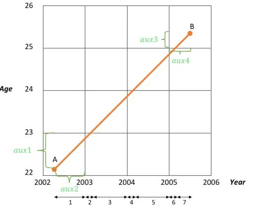
As a simple illustration, consider a player, who was born on 15 February 1980, enters the study on 5 April 2002 and leaves the study on 14 June 2005. Therefore, he starts to be followed with 22.13 years (point A) and his age at exit will be 25.33 years (point B). Considering age-class and calendar period of one year, he contributes with observation times to seven different categories, as shown in Figure 3.1.
The exposed to risk of each category equals the corresponding width of the lattice at the bottom. Since the two variables in the axes have the same scale, only four different values of exposed to risk need to be calculated, namely, the first and the last widths of the lattices (in the example, 1 and 7, respectively); the value of the lattices with even numbers and the value of the lattices with odd numbers.
Define 𝑊𝐼𝐷𝑇𝐻 as the width of each variable in the axis and consider 𝑎𝑢𝑥1, 𝑎𝑢𝑥2, 𝑎𝑢𝑥3 and 𝑎𝑢𝑥4 as illustrated in Figure 3.1.
11 Figure 3.1 – Lexis diagram divided into 1x1 cells (one year of age by one year of time) to illustrate the follow-up of a hypothetic individual and the computation of his exposure to risk.
The property of the sum of neighbor widths being equal to the scale of the original variables (𝑊𝐼𝐷𝑇𝐻), unless one of them is the first or the last lattice, allows determining the population at risk:
𝑤𝑖𝑑𝑡ℎ1 = 𝑚𝑖𝑛 {𝑎𝑢𝑥1, 𝑎𝑢𝑥2}
𝑤𝑖𝑑𝑡ℎ2 = |𝑎𝑢𝑥1 − 𝑎𝑢𝑥2|(= 𝑤𝑖𝑑𝑡ℎ4 = 𝑤𝑖𝑑𝑡ℎ6) 𝑤𝑖𝑑𝑡ℎ3 = 𝑊𝐼𝐷𝑇𝐻– 𝑤𝑖𝑑𝑡ℎ2(= 𝑤𝑖𝑑𝑡ℎ5)
𝑤𝑖𝑑𝑡ℎ7 = 𝑚𝑖𝑛 {𝑎𝑢𝑥3, 𝑎𝑢𝑥4}
The individual contribution to the exposed to risk by this athlete is summarised in Table 3.1, where values are in days. Notice that the output obtained when using software may be different, since some adjustments are usually performed to consider leap years and assumptions about the date of entry and exit are made, namely, whether they count for the observed time.
Age Calendar year
2002 2003 2004 2005
22 271 45
23 320 45
24 320 45
25 120
Table 3.1 – Central exposed to risk (in days) by age and calendar year for the hypothetic individual
Age Year 26 25 24 23 22 2002 2003 2004 2005 2006 1 2 3 4 5 6 7 𝑎𝑢𝑥4 𝑎𝑢𝑥1 𝑎𝑢𝑥2 A B 𝑎𝑢𝑥3
12
The computation of exposed to risk is crucial for evaluating the following mortality measures.
3.1.3 Crude Mortality Rate (CMR)
The crude (non-standardised) mortality rate for a particular population is the total number of deaths observed during the period divided by the total exposed to risk for the same period.
𝐶𝑟𝑢𝑑𝑒 𝑚𝑜𝑟𝑡𝑎𝑙𝑖𝑡𝑦 𝑟𝑎𝑡𝑒 = ∑ 𝐸𝑗 𝑚𝑗 𝑀 𝑗=1 ∑𝑀 𝐸𝑗 𝑗=1 (1)
This rate can be calculated just for a certain category, for example, as the ratio of total number of deaths in one age-class to the total exposed to risk in the same age-class.
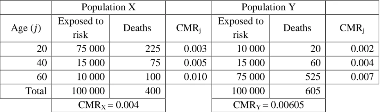
Comparing crude mortality rates of different populations might give a misleading result, since the measure does not take into account differences in their demographic structures. In particular, the crude mortality rate disregards the age structure of the population. If one population is, on average, younger than the other, then, even if the age-specific rates were the same in both populations, more deaths would occur in the older population than in the younger, considering exactly the same period of observation. Actually, given higher crude mortality rates in a population X at each age-class than in a population Y, it is possible to obtain a lower overall crude mortality for population X, as illustrated in the example below.
Population X Population Y Age (𝑗) Exposed to risk Deaths CMRj Exposed to risk Deaths CMRj 20 75 000 225 0.003 10 000 20 0.002 40 15 000 75 0.005 15 000 60 0.004 60 10 000 100 0.010 75 000 525 0.007 Total 100 000 400 100 000 605 CMRX = 0.004 CMRY = 0.00605
Table 3.2 – Example of computation of CMR to illustrate that this measure can be misleading if used to compare the two populations. Adapted from:IFOA (2011), Core Reading: Subject CT5, Chapter 15.
A valid comparison is obtained when the mortality rate is recomputed by assuming the same age structure in the two populations, which is one form of standardisation, as already mentioned.
There are two types of standardisation, direct and indirect, both requiring assumption of a standard or reference population.
13
3.1.4 Directly Standardised Mortality Rate (DSMR)
The directly standardised mortality rate is obtained by applying the stratum-specific cohort mortality rates to the standard population distribution. More formally:
𝐷𝑆𝑀𝑅 = ∑ 𝐸𝑗 𝑠 𝑚 𝑗 𝑀 𝑗=1 ∑ 𝑠𝐸 𝑗 𝑀 𝑗=1 (2)
This measure can be regarded as a weighted average of the stratum-specific cohort mortality rates, with the weights being the stratum-specific proportions in the standard population, 𝑠𝑤𝑗 = 𝐸 𝑠 𝑗 ∑𝑀𝑗=1 𝑠𝐸𝑗 :
(3) 𝐷𝑆𝑀𝑅 = ∑ 𝑤𝑠 𝑗𝑚𝑗 𝑀 𝑗=1 (4)
If the standardisation is only by age, the directly standardised mortality rate is the number of deaths that would have occurred in the standard population if it had the age-specific mortality of the cohort, divided by the total central exposed to risk of the standard population. Provided that the same reference population is used in the standardisation, computation of directly standardised rates is expected to provide a meaningful comparison between the mortality experience of different cohorts, by eliminating the effect of different age structures. However, the standard population affects this measure, so it should be chosen carefully.
3.1.5
Indirectly Standardised Mortality Rate (ISMR)
The indirectly standardised mortality rate is defined as the crude mortality rate for the standard population multiplied by the ratio of actual to expected deaths in the cohort, as follows: 𝐼𝑆𝑀𝑅 =∑ 𝐸𝑗 𝑚𝑗 𝑠 𝑠 𝑀 𝑗=1 ∑𝑀 𝑠𝐸𝑗 𝑗=1 × ∑ 𝐸𝑗 𝑚𝑗 𝑀 𝑗=1 ∑𝑀 𝐸𝑗 𝑠𝑚𝑗 𝑗=1 (5)
The rate can also be decomposed as: 𝐼𝑆𝑀𝑅 = 𝐹 x CMR for population under study ,
where 𝐹 = ∑𝑀𝑗=1 𝑠𝐸𝑗 𝑚𝑗𝑠 ∑𝑀𝑗=1 𝑠𝐸𝑗 ∑𝑀𝑗=1𝐸𝑗𝑠𝑚𝑗 ∑𝑀𝑗=1𝐸𝑗 = 𝐶𝑟𝑢𝑑𝑒 𝑚𝑜𝑟𝑡𝑎𝑙𝑖𝑡𝑦 𝑟𝑎𝑡𝑒 𝑓𝑜𝑟 𝑠𝑡𝑎𝑛𝑑𝑎𝑟𝑑 𝑝𝑜𝑝𝑢𝑙𝑎𝑡𝑖𝑜𝑛 𝐶𝑟𝑢𝑑𝑒 𝑚𝑜𝑟𝑡𝑎𝑙𝑖𝑡𝑦 𝑟𝑎𝑡𝑒 𝑓𝑜𝑟 𝑐𝑜ℎ𝑜𝑟𝑡, 𝑢𝑠𝑖𝑛𝑔 𝑠𝑡𝑎𝑛𝑑𝑎𝑟𝑑 𝑚𝑜𝑟𝑡𝑎𝑙𝑖𝑡𝑦 (6)
is the Area Comparability Factor. A value of 𝐹 greater than 1 indicates that the structure of the population being studied is more heavily weighted towards individuals who experience lighter mortality than the standard population.
14
Usually, the indirectly standardised mortality rate gives a good approximation to the directly standardised mortality rate and it is often more easily calculated, since it is not necessary to know the stratum-specific mortality rates of the cohort (only the total number of deaths).
It is possible to take important conclusions from the last single figure indices: - If the DSMR, the ISMR and the crude mortality rate for the standard population are greater
than the crude mortality rate for the studied population, then, the reason for the lower mortality rate of the cohort is its population distribution (by the variables being used in the standardisation);
- If the crude rate for the standard population is greater than both the DSMR and ISMR, the crude rate for the studied population is lower, even allowing for the population distribution.
3.1.6
Standardised Mortality Ratio (SMR)
The standardised mortality ratio has been one of the most used summary mortality measures. The SMR compares the observed number of deaths in the population being studied with the expected number of deaths obtained by applying the stratum-specific mortality rates of the standard population to the corresponding population at risk in the cohort.
It is formally defined as: 𝑆𝑀𝑅 = ∑ 𝐸𝑗𝑚𝑗 𝑀 𝑗=1 ∑𝑀𝑗=1𝐸𝑗 𝑠𝑚𝑗= ∑𝑀𝑗=1𝑑𝑗 ∑𝑀𝑗=1𝐸𝑗 𝑠𝑚𝑗 = 𝑎𝑐𝑡𝑢𝑎𝑙 𝑑𝑒𝑎𝑡ℎ𝑠 𝑖𝑛 𝑡ℎ𝑒 𝑐𝑜ℎ𝑜𝑟𝑡 𝑒𝑥𝑝𝑒𝑐𝑡𝑒𝑑 𝑑𝑒𝑎𝑡ℎ𝑠 𝑖𝑛 𝑡ℎ𝑒 𝑐𝑜ℎ𝑜𝑟𝑡 (7) Notice that the indirectly standardised mortality rate is obtained multiplying the crude mortality rate of the standard population by the SMR.
One advantage of the SMR is that specific numbers of deaths (or stratum-specific mortality rates) in the cohort are not required for its calculation, only the total number of deaths. This allows application of the SMR to published data which omits details on the number of deaths by subgroup but gives information about the population at risk.
A value of the SMR lower than 1 indicates that the study population exhibits lower mortality than the standard population, and vice-versa.
Besides estimating the SMR, one question of interest is its statistical significance. The hypothesis test and the determination of confidence intervals are explained in the Appendix. This summary statistic is widely used in studies on mortality and longevity of elite athletes, engaging in different types of sports:
- An overall SMR of 0.59 shows a substantially and significantly lower mortality in French participants in the Tour de France compared with the general French male population
15
(Marijon et al., 2013). Cyclists are also grouped in the intervals 1947-70, 1971-90 and 1991-2010, according to their participation in Tour de France. The reason behind this is to address (indirectly) the possible effect of doping on long-term mortality and to account for mortality trends. For the first two periods, it is observed a 41% and 32% lower mortality in French cyclists, while no deaths are recorded in the last period. It is also taken into account a possible age period interaction, again resulting in SMR lower than 1, without any significant difference over time. Reduction in mortality is also verified for major causes of death, which are neoplasms (SMR: 0.56) and cardiovascular diseases (SMR: 0.67). The exception is mortality associated to external causes (mainly, trauma-related), with no clear difference between cyclists and the general population.
- Taioli (2007) concluded that the SMR of the cohort of professional soccer players enrolled in Italian A and B leagues from 1975 to 2003 is 0.68, based on age and calendar-period stratified mortality from the general male population in Italy. However, a significantly higher than expected number of deaths for ALS and car accidents was observed, giving SMR of 18.18 and 2.23, respectively.
- The mortality experience of Major US league baseball players is found to be lower than that of the reference population in several studies. For example, Kalist and Peng (2007) observe an actual number of deaths 69% lower than the expected (SMR=0.31), for players born between 1945 and 1964; Reynolds and Day (2012) compute a SMR which is higher but still significantly lower than 1 (SMR=0.87) for the 1930-1999 period.
- In another study including the Polish athletes participating in the twentieth century Olympics since 1924, the SMR is 0.5 for males and 0.73 for females, using as standard population the urban Polish males, and females, respectively, also stratifying by age (Gajewski and Poznańska, 2008).
- Danish athletic champions, record-holders and members of national teams from 19 different sports, born in the calendar-period 1880-1910, are divided in three age-classes in a study conducted by Schnohr (1971). The male elite athletes had a significantly lower mortality than the standard population under the age of 50 years (SMR=0.61 in the life period 25-49 years), while the actual deaths were not significantly different from the expected deaths after 50 years old (SMR=1.08 in 50-64 years and SMR=1.02 in 65-80 years).
The standardised mortality ratio is also used to evaluate morbidity rates, being known in this context as standardised incidence ratio (SIR), a summary statistic that assesses the risk associated with a specific disease. The SMR and SIR are particularly applicable when the population under study is so small, or the event of interest is rare, that the resulting stratum-specific rates are not stable.
16
3.2
Observed and expected survival function
Besides providing single summary measures of mortality, it is useful to compare two (or more) populations based on the estimation of their survival functions.
The survival function is defined as 𝑆(𝑡) = 𝑃(𝑇 > 𝑡) = 𝑝𝑡 0 and represents the probability that an individual at time or age 0 survives at least 𝑡 years. On the other side, the lifetime distribution function from time or age 0 is defined as 𝐹(𝑡) = 1 − 𝑆(𝑡) = 𝑃(𝑇 ≤ 𝑡) =
𝑞0
𝑡 , and represents the probability that the individual does not survive beyond time or age 𝑡.
3.2.1 Kaplan-Meier method – Estimation of observed survival
The Kaplan-Meier estimator of the survival function is one of the most widely used methods for statistical comparison and graphic display of survivorship over time, not requiring a functional form for the survival function (non-parametric).
Individuals in the cohort are followed from their entry into study until they die, withdraw from the investigation while still alive or reach the time of end of the investigation, whichever of these three events occurs first. These last two situations are examples of right censoring, which plays an important role in estimating survival rates.
In the next presentation of the Kaplan-Meier method (Klugman, Panjer and Willmot, 2008) lifetimes will be considered as a function of time 𝑡,without mention of a starting age 𝑥. Suppose the population under study is composed of N individuals, in the presence of non-informative censoring, and d deaths are observed. Then, 𝑁 − 𝑑 lives are censored. Let:
• 𝑡1< 𝑡2< … < 𝑡𝑘 , 𝑘 ≤ 𝑑, be the ordered times at which deaths are observed.
Define 𝑡0 = 0 ;
• 𝑑𝑗 denote the number of deaths at time 𝑡𝑗 (𝑗 = 1, … , 𝑘) , with 𝑑𝑗≥ 1 ( 𝑑 = ∑𝑘 𝑑𝑠
𝑠=1 );
• 𝑟𝑗, known as the risk set, denote the number of individuals alive and uncensored at
𝑡𝑗− (𝑗 = 1, … , 𝑘);
• 𝑐𝑗 denote the number of individuals censored in the interval [𝑡𝑗 , 𝑡𝑗+1[ (0 ≤ 𝑗 ≤ 𝑘 − 1).
Therefore, 𝑟1 = 𝑁 − 𝑐0 and 𝑟𝑗= 𝑁 − ∑𝑠=1𝑗−1𝑑𝑠− ∑𝑗−1𝑠=0𝑐𝑠 , 2 ≤ 𝑗 ≤ 𝑘. ⇒ 𝑟𝑗= 𝑟𝑗−1− 𝑑𝑗−1− 𝑐𝑗−1 , 2 ≤ 𝑗 ≤ 𝑘.
It can be shown that the Kaplan-Meier estimate, 𝑆̂(𝑡), is a monotonically non-increasing step function and is obtained by multiplying the survival probabilities,
𝑛𝑢𝑚𝑏𝑒𝑟 𝑜𝑓 𝑠𝑢𝑟𝑣𝑖𝑣𝑜𝑟𝑠 𝑎𝑡 𝑡𝑗
17 1 , 𝑡 < 𝑡1 𝑆̂(𝑡) = ∏𝑟𝑠− 𝑑𝑠 𝑟𝑠 𝑗−1 𝑠=1 , 𝑡𝑗−1≤ 𝑡 < 𝑡𝑗 (8) ∏𝑟𝑠− 𝑑𝑠 𝑟𝑠 𝑘 𝑠=1 𝑜𝑟 0 , 𝑡 > 𝑡𝑘
3.2.2
Estimation of expected survival
The expected survival function is estimated to provide a comparison between the survival of the population of elite athletes and the standard population. The most common approaches are the exact method, the cohort method and the conditional expected survival. These three methods differ in how long the athlete’s counterpart in the standard population is considered to be at risk for the calculation of the expected survival.
The exact method, also known as Ederer I method (Ederer, Axtell and Cutler, 1961), assumes a complete follow-up for all athletes; consequently, the matched individuals are considered to be at risk indefinitely. There is a technical problem with this method, since it often requires standard population data that is not yet available, namely, for the younger individuals under study.
The conditional expected survival, known as Ederer II method (Ederer and Heise, 1959), is based on the actual follow-up time, therefore, matched individuals are considered to be at risk only until the corresponding athletes die or are censored.
The cohort method, proposed by Hakulinen (Hakulinen, 1982), takes into account potential follow-up time, which is the maximum possible time that an individual can be followed-up from the date of entry into study to the last potential time of observation. Explicitly, if the study subject is censored, the matched referent is assumed to be no longer at risk (actual follow-up), but if he dies, the counterpart is considered to remain at risk (maximum potential follow-up).
In the following (Pokhrel, 2007; Therneau and Offord, 1999), brief formulae for the estimation of expected survival by each method is given, applying, for simplicity, the convention that both the begin date and the end of follow-up occurred on an individual’s birthday. Again, lifetimes will be considered as a function of time 𝑡 (𝑡 ≥ 0).
Let 𝒑𝒊𝒌𝒔 be the annual conditional expected survival probability of a corresponding person in the standard population similar to the 𝑖𝑡ℎ athlete, with respect to age and calendar
year of entry into study. The expected probabilities for individual 𝑖, obtained from the standard life tables, can be summarized as follows (Table 3.3).
18
Interval Age Calendar year 𝑝𝑖𝑘𝑠
[0,1[ a y 𝑝𝑖1𝑠
[1, 2[ a+1 y+1 𝑝𝑖2𝑠
… … … …
Table 3.3 – Illustration of age and calendar year specific annual survival probabilities.
The expected probability of individual 𝑖 surviving until the end of interval [𝑡 − 1, 𝑡[ is then obtained by the product:
𝑆𝑖𝑠(𝑡) = ∏ 𝑝𝑖𝑘𝑠 𝑡
𝑘=1
(9)
Exact method
The cumulative expected survival probability from beginning of study to the end of interval [𝑡 − 1, 𝑡[ is estimated by: 𝑆̃(𝑡)𝐸𝐼 = 1 𝑙1∑ (∏ 𝑝𝑖𝑘 𝑠 𝑡 𝑘=1 ) 𝑙1 𝑖=1 = 1 𝑙1∑ 𝑆𝑖 𝑠(𝑡) 𝑙1 𝑖=1 , (10)
where 𝑙1 is the number of individuals at risk at the start of the first interval (which is equivalent to 𝑁, defined in section 3.2.1). Therefore, the estimate by the exact method is an average of the cumulative expected survival probabilities of all individuals who enter into study.
Conditional expected survival
The first step in Ederer II method consists in calculating the annual survival probabilities for each interval [𝑘 − 1, 𝑘[: 𝑝∗𝑘𝑠 = 1 𝑙𝑘∑ 𝑝𝑖𝑘 𝑠 𝑙𝑘 𝑖=1 (𝑘 = 1,2, … ), (11) where 𝑙𝑘 is the number of individuals at risk (alive and not censored) at the start of interval [𝑘 − 1, 𝑘[. The next and final step is obtaining the estimate of the survival function at time 𝑡:
𝑆̃(𝑡)𝐸𝐼𝐼 = ∏ (1 𝑙𝑘 ∑ 𝑝𝑖𝑘𝑠 𝑙𝑘 𝑖=1 ) 𝑡 𝑘=1 = ∏ 𝑝∗𝑘𝑠 (12) 𝑡 𝑘=1 Cohort method
The cohort method for the estimation of the expected survival function was initially proposed by Hakulinen (1982).
19
After specifying the potential follow-up times for all individuals, let consider a generic interval [𝑘 − 1, 𝑘[. From the group of individuals with potential follow-up greater or equal to 𝑘 − 1, define two subgroups: 𝛼𝑘 having a potential follow-up greater or equal to 𝑘 and 𝛽𝑘 having a potential follow-up less than 𝑘. The latter are, in effect, those who withdraw during the interval. An expected life table can be built considering:
- the expected number of individuals alive and under observation at time 𝑘 − 1: 𝑙𝑘∗ = {
𝑙1 , 𝑖𝑓 𝑘 = 1 ∑ 𝑆𝑖𝑠(𝑘 − 1)
𝑖∈𝛼𝑘−1
, 𝑖𝑓 𝑘 ≥ 2 (13) - the expected number of deaths among the 𝛼𝑘 group during interval [𝑘 − 1, 𝑘[:
𝑑𝑘∗ = { ∑ [1 − 𝑝𝑖𝑘𝑠] 𝑖∈𝛼𝑘 , 𝑖𝑓 𝑘 = 1 ∑ 𝑆𝑖𝑠(𝑘 − 1) × [1 − 𝑝𝑖𝑘𝑠] , 𝑖𝑓 𝑘 ≥ 2 𝑖∈𝛼𝑘 (14)
- the expected number of individuals withdrawing alive during interval [𝑘 − 1, 𝑘[:
𝑤𝑘∗ = { ∑ √𝑝𝑖𝑘𝑠 𝑖∈𝛽𝑘 , 𝑖𝑓 𝑘 = 1 ∑ 𝑆𝑖𝑠(𝑘 − 1) × √𝑝𝑖𝑘𝑠 𝑖∈𝛽𝑘 , 𝑖𝑓 𝑘 ≥ 2 (15)
- the expected number of deaths among the 𝛽𝑘 group, during interval [𝑘 − 1, 𝑘[:
𝜎𝑘∗ = { ∑[1 − √𝑝𝑖𝑘𝑠] 𝑖∈𝛽𝑘 , 𝑖𝑓 𝑘 = 1 ∑ 𝑆𝑖𝑠(𝑘 − 1) × [1 − √𝑝𝑖𝑘𝑠] 𝑖∈𝛽𝑘 , 𝑖𝑓 𝑘 ≥ 2 (16)
- the total expected number of deaths during interval [𝑘 − 1, 𝑘[:
𝐷𝑘∗ = 𝑑𝑘∗ + 𝜎𝑘∗ (17) Then, the expected interval-specific survival probability is estimated using the actuarial (life table) approach:
𝑝∗𝑠(𝑘) = 1 − 𝐷𝑘∗
𝑙𝑘∗− 𝑤𝑘
∗
2
(18)
Finally, the expected cumulative survival from the beginning of the first interval to the end of interval [𝑡 − 1, 𝑡[ by the Hakulinen method, is given by:
𝑆̃(𝑡)𝐻= ∏ 𝑝 ∗𝑠(𝑘) 𝑡
𝑘=1
20
3.3 Years of Life Lost/Saved
Most of the studies included in literature review use indirect standardisation of elite athletes’ mortality to assess the difference in mortality between two populations or, otherwise, to conclude that there is no statistically significant difference between them. As already mentioned, the clear majority found a greater survival of elite athletes when compared to the general population. While this is a useful approach in mortality comparison and a valuable way to give a background to new research, it may not be straightforward to interpret. For example, a 30% lower mortality is better than a 20% lower mortality, but what does a 10% difference mean in terms of life duration?
A possible tool to provide a time dimension measure for athletes’ longevity is determining the number of years of life lost (YLL) in case of shorter longevity than the standard population, or saved, otherwise. The years lost method, as proposed by Andersen (2013), quantifies the expected number of years of life lost due to a given cause of death before a certain age. It has been primary developed to be applied in studies of cancer patients.
In sports, the overall years lost/saved is obtained as a stand-alone measure of mortality. In addition, it is often determined for each major cause of death, as well as according to the main type of physiological effort, allowing comparisons between groups (Antero-Jacquemin J, 2018).
The determination of YLL (Andersen, 2013) requires the definition of the following measures.
- Life expectancy at time 0: 𝑒0= ∫0∞ 𝑡𝑝0𝑑𝑡 (20) - Temporary life expectancy, also known as restricted mean life time, between 𝑡 = 0
and 𝑡 = 𝑥: 𝑒𝑥 0= ∫ 𝑡𝑝0 𝑥
0 𝑑𝑡 (21)
The life expectancy at time 0, 𝑒0, corresponds to the area under the survival curve, while 𝑥𝑒0 is the area under the curve until the given threshold 𝑡 = 𝑥.
Noticing that the equation 𝑡𝑝0+ 𝑞𝑡 0= 1 holds, and integrating it from 𝑡 = 0 to 𝑡 = 𝑥, another balance equation is obtained:
𝑒0 𝑥 + ∫ 𝑡𝑞0 𝑥 0 𝑑𝑡 = 𝑥 , (22) where ∫𝑥 𝑡𝑞0
21
Rearranging equation (22), 𝑌𝐿𝐿(0, 𝑥) is obtained by subtracting temporary life expectancy from 𝑥:
𝑌𝐿𝐿(0, 𝑥) = 𝑥 − 𝑒𝑥 0 (23)
Graphically, it corresponds to the area above the survival curve, 𝑦 = 𝑆(𝑡), and below the horizontal line at 1, 𝑦 = 1, from 𝑡 = 0 to 𝑡 = 𝑥. Equivalently, this is the area under the lifetime distribution function 𝐹(𝑡), until 𝑡 = 𝑥.
Finally, the years of life lost method can be used to compare life expectancies between two populations. Temporary life expectancy can be expressed as a function of the total number of years and the number of years lost. For example, for country 𝑐1:
𝑒0 𝑥 𝑐1 = 𝑥 − ∫ 𝑞 0 𝑡 𝑐1 𝑥 0 𝑑𝑡 , (24) and then the difference between the life expectancies of two populations can be obtained by looking at their years lost as:
𝑒0 𝑥 𝑐1 − 𝑒 0 𝑥 𝑐2 = ∫ 𝑞 0 𝑡 𝑐2 𝑥 0 𝑑𝑡 − ∫ 𝑐𝑡1𝑞0 𝑥 0 𝑑𝑡 ⟺ 𝑐𝑥1𝑒0− 𝑒 0 𝑥 𝑐2 = 𝑌𝐿𝐿 𝑐2(0, 𝑥) − 𝑌𝐿𝐿𝑐1(0, 𝑥) (25) If 𝑐𝑥1𝑒0> 𝑒 0 𝑥 𝑐2
, the total number of years lost before 𝑥 is larger in population 𝑐2 than in 𝑐1. Under the context of this work, denoting 𝑐1 as the group under study and 𝑐2 as the standard population, if the difference in (25) is positive it represents the survival gain, in terms of years saved, of the group of athletes in comparison to the standard population. Otherwise, a negative result in (25) estimates the number of years lost in the group of athletes in relation to the standard population.
The same methodology can be applied when estimating the years saved/lost from a certain cause of death, following the competing risk model (Andersen, 2013), through the replacement of the overall probabilities of dying by the cumulative incidence functions for a specific cause.
Notice that all the quantities presented can be defined conditionally on survival until time 𝑡 = 𝑥. For instance, the temporary life expectancy between times 𝑥 and 𝑥 + 𝑛 is:
𝑒𝑥
𝑛 = ∫ 𝑡 𝑥𝑝 𝑛
0 𝑑𝑡 . Furthermore, time can be interpreted as age. More details can be found in
22
3.4 Cox Proportional Hazard Models
In addition to comparing the mortality of elite athletes with that of a standard population, it is also interesting to analyse if there are mortality differences inside the group of athletes, resulting from having different characteristics. For example, it can be investigated if mortality of a team player (football, baseball, etc.) is influenced by his/her position on the field.
Cox Proportion Hazard Model (Cox, 1972) is applicable in this context, besides being one of the most widely used tools of survival analysis. The quantity that plays a central role in this model is the hazard rate, also known as force of mortality, and defined as:
𝜆(𝑡) = lim
ℎ→0
1
ℎ𝑃(𝑇 ≤ 𝑡 + ℎ | 𝑇 > 𝑡) , (26) where 𝑇 is the random variable representing the future lifetime at time 0. The hazard rate is an instantaneous measure of mortality at time 𝑡 and fully describes the lifetime distribution (as the survival distribution does). If the time scale is age, the hazard rate is usually represented as 𝜆(𝑥) and 𝑇 is the future lifetime at birth.
In the Cox Proportional Hazard Model, the hazard rate takes the form:
𝜆(𝑡, 𝒛) = 𝜆0(𝑡)𝑒𝜷𝒛𝑇 , (27)
where 𝒛 is a vector of covariates, which are the different factors used to split the population under study into homogeneous subgroups; 𝜷 is a vector of regression parameters and 𝜆0(𝑡) is the baseline hazard (all 𝒛𝒊 = 0), a function of time 𝑡 and independent of the covariates.
This is a semi-parametric model since the baseline hazard is unspecified, that is, no assumptions are made about the shape of 𝜆0(𝑡) before analysing the data.
Noticing that the hazards of different individuals with covariate vectors 𝒛𝟏 and 𝒛𝟐 are in the same proportion at all times:
𝜆(𝑡, 𝒛𝟏) 𝜆(𝑡, 𝒛𝟐)=
𝑒𝜷𝒛𝟏𝑇
𝑒𝜷𝒛𝟐𝑇 = 𝑐𝑜𝑛𝑠𝑡𝑎𝑛𝑡 , (28)
Cox regression belongs to the category of proportional hazard models.
Since the aim of the analysis is to compare mortality across different groups, 𝜆0(𝑡)
can be “ignored”. Then, the vector 𝜷 is estimated from the data, through the maximisation of the partial likelihood function and assuming a method (e.g. Breslow’s approximation) to handle deaths that occur at the same time. For more details, cf. IFOA (Subject CT4, 2011).
The Cox Proportional Hazard Model is fitted in software R with the coxph function, belonging to the package survival.
23
In the literature, there are several works that have used the Cox Proportional Hazard technique to analyse the effect of specific variables in mortality of athletes, as already mentioned in Chapter 2. Here, it should be emphasised that most of them use the age attained by the athlete at entry into study as the relevant time scale, allowing for censored observations (Zwiers et al., 2012; Baron et al., 2012; Koning et al., 2014). Alternatively, follow-up time can be chosen, though being an approach primarily used in epidemiological studies.
The covariates used vary from study to study, depending on the characteristics of the sport, the data availability and the main objective of the research. While Koning et al. (2014) focused on overall mortality of NFL players, examining whether observable factors as number of games played, position played and race, influence the individual risk of mortality, Baron et al. (2012) studied the association of NFL players position category and BMI with cardiovascular disease mortality. Targeting a broader group of elite athletes, those who participated in the Olympic Games between 1896 and 1936, Zwiers et al. (2012) determined hazard ratios for all-cause mortality dependent on different levels of exercise intensity, risk of bodily collision and levels of physical contact.
Besides mortality, Cox Proportional Hazard Models were also used to assess disability relative risks. One example is the study based on a cohort of male Finnish elite athletes (Sarna et al., 1997) evaluating the association between the type of sport – endurance athletes, team games and power sports – with specific disabilities.
The models are usually adjusted for other variables, as race, era of play, time since last game played and calendar year of follow-up (by decades) in Baron et al. (2012); sex, year of birth and nationality in Zwiers et al. (2012), and marital status and social class in Sarna et