The MNP distribution in the subject can be determined by solving the inverse problem in the forward modelKc= y. In this thesis, the OED is determined with regard to the placement of the instruments.
Imaging Setup
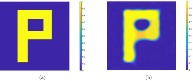
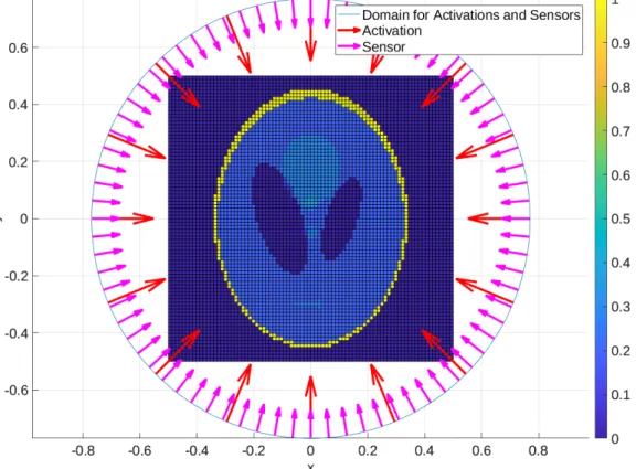
By solving the inverse problem associated with MRXI, a reconstruction of the particle distribution can be made. The actual particle distribution has the shape of the letter P and it is shown on the left.
Forward Model
The sensor measures the amplitude of the magnetic field generated by the MNPs in the ROI. Since the MNP density c(rd) is the quantity of interest, all other parameters in (4) can be included in the system matrix of the MRXI forward model.

Estimators
For the posterior covariance, the new definition only requires the inversion of the matrix Γnoise+KΓprKT ∈Rm×m. In the numerical experiments of this thesis, the reconstructions of the MNP distribution are given as the mean of the posterior distribution.
D-Optimality
For example, in A the dimensions of the finite elements can be taken into account. Moreover, if the reconstruction quality is not important in some regions of the ROI, it can be expressed in A. In this thesis, A is the identity matrix, since the reconstruction quality is considered equally important everywhere and the finite elements are equal in size. Since the trace is linear and invariant under cyclic permutations, the objective function simplifies to .
This is done by using some properties of conditional distributions and changing the order of integration (remember that x does not depend on η). If the distributions are Gaussian, Shannon's (1948) explicit representation for entropy can be used. Finally, the simplified version for the objective function is obtained by combining the new forms for the two terms: .
Thus, it suffices to represent the objective function as 17) The logarithm in (17) follows from the definition of D-optimality and also makes the numerical evaluation of ΦD more stable for large matrices.
Gaussian Prior
The algorithm to find the optimal design parametersη with respect to the Gaussian prior is shown in Algorithm 1. Additionally, design the sensor setup with Ns sensors and initialize the actuation positioning for optimization.
Edge-Promoting Priors
Total Variation Prior
Consequently, the use of the optimization methods considered in this thesis, namely, gradient descent and Newton's method, become inapplicable for finding a MAP estimate for the MRXI inverse problem. Therefore, there are two issues that prevent the use of advance as is. The differentiability issue is solved by an approximation and the non-Gaussian nature of the prior is handled using delayed diffusivity iteration.
Furthermore, yk is the measurement vector of previous measurements, Kkis the system matrix corresponding to the previously optimized activations, and Γ(k)noise is the noise covariance matrix, which is determined by the noise covariance matrices of the previously taken measurements. Specifically, it allows the use of the objective functions derived for A- and D-optimality in sections 4.1 and 4.2. Before considering the delayed diffusivity iteration, a Gaussian approximation is needed for the prior around ck−1, where k is the index of the sequentially optimized activation.
The gradient of R(c) is obtained with. 21) The positive definiteness and thus the invertibility of H(c) is guaranteed by the Poincaré-Friedrich inequality (Braess, 2001).
Perona-Malik Prior
The node basis functions are defined such that in the center of pixel j in the ROI the node basis function j has value one and in the center of other pixels has value zero. As can be seen from (22) and (23), the differentiability of the term R(c) is not a problem with the Perona-Malik prior. As with the earlier TV, the delayed diffusion iteration is used to solve this problem.
The gradient of R(c) is thus obtained with . 24) The invertibility of H(c) is again guaranteed by means of the Poincaré-Friedrichs inequality (Braess, 2001).
Lagged Diffusivity Iteration
This covariance matrix is used to select the next optimal design parametersηk+1, i.e. the location and orientation of the next activation. Since the methods are derivative-based, the partial derivatives of the objective functions are necessary. In magnetorelaxometric imaging, the design parametersη often correspond to the location of the actuation and magnetic field sensors.
The configuration in the figure serves as the basis for the optimization process of the Bayesian experimental design implemented in this thesis. It is used for matrix Z, because its inverse is needed for the evaluation of the partial derivative of the objective function. In addition to the first-order derivatives, Newton's method requires the calculation of the Hessian matrix of the objective function.
The design parameters consist of the polar angles corresponding to the location and orientation of each actuation.
Gradient Descent
Consequently, Newton's method requires the calculation of 3×Na separate nonzero second-order partial derivatives of K(η). The second-order partial derivatives are not included here to keep this section concise. However, its derivation can be easily done by differentiating the first-order partial derivatives provided above.
The step size can be determined heuristically or by using an algorithm in each iteration. The gradient descent algorithm for minimizing the objective function value with respect to design parametersη is described in Algorithm 3. At each step, the search direction is determined as the normalized negative gradient of the objective function ΦA evaluated at the previous design parameters ηi.
The optimal step size is then selected using the step size determination algorithm presented in Section 5.4.
Newton’s method
The Hessian matrix in (34) must be positive definite, since otherwise the search direction given by Newton's method may be an ascent direction in the value of the objective function. The method used here is based on the idea of adding a multiple of the identity matrix to the Hessians, which need to be modified. One decides a positive scalarτ such that Hf +τ I is sufficiently positive definite, where I is the identity matrix (Nocedal & Wright, 1999).
The algorithm for minimizing the objective function value with respect to design parameters η using Newton's method is described in Algorithm 5. At step i, the search direction di is determined as −HΦA(ηi)−1∇ΦA(ηi), where ηi describes the design parameters at step i. Again, the optimal step size is determined based on the step size determination algorithm presented in Section 5.4.
Determining the Step Size for the Optimization Methods
Analysis on the Objective Function
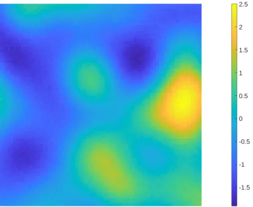
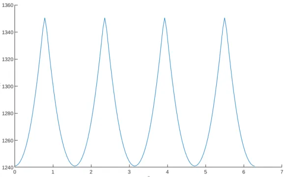
The activation location domain and the orientation angle domain, i.e. the circle with radius r= 0.77 and [0.2π), are both divided into 128 segments. With this discretization, there are a total of 128×128 different positions tested for the activation. A surface plot of the objective function values at 128×128 actuation positions can be seen in Figure 9. It is clear that patterns in the objective function repeat at an interval of π in the orientation angle γ.
Polar angles corresponding to orientation and location can be seen on the x and y axes, respectively. In this plot, the polar angle of the activation location is varied and its orientation is fixed to be towards the center of the ROI. In other words, since a Gaussian prior is used in the experiments, the measurements have no effect on the Bayesian experimental design.
With this setup, the orientation angle γ is fixed to point towards the center of the ROI.

Optimization Performance
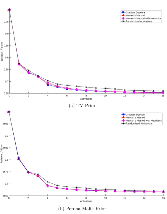
In the figure, the expected reconstruction errors correspond to the averages of 10 runs of the algorithms. In any case, the use of the optimization methods seems to provide an improved experimental design compared to randomized activation placements alone. The running times of the algorithms can be seen in Table 1. These times correspond to a single run of the optimization algorithms.
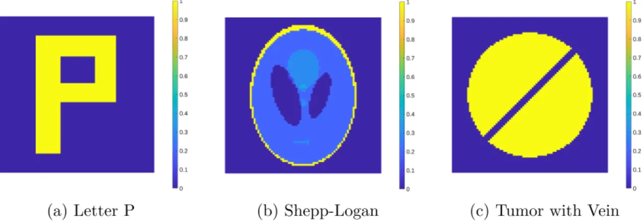
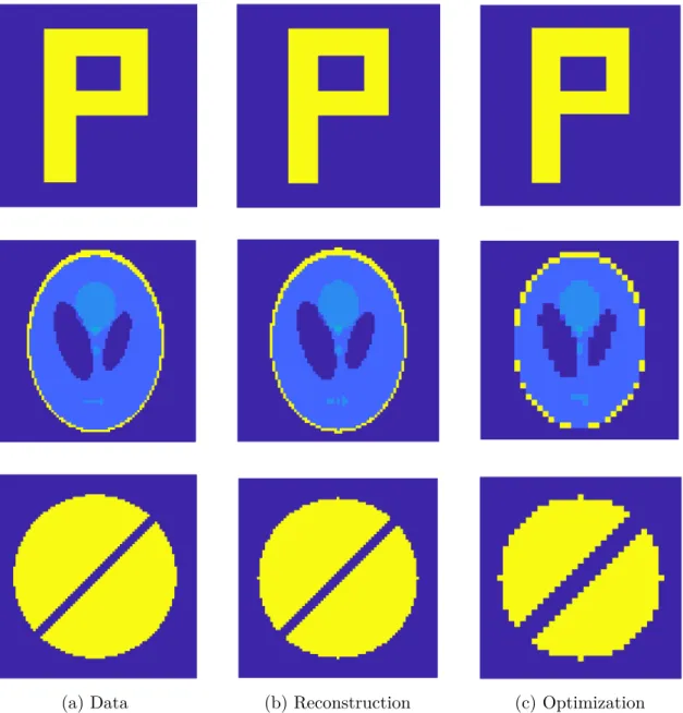
Reconstructions of the three phantoms with a Gaussian prior can be seen in Figure 13. The letter P reconstruction has the best quality compared to the underlying MNP distribution. In addition, the edges become blurred and practically all the features of the interior are lost during the reconstruction.
There is one key feature that can be seen when comparing the reconstructions in Figure 13 with the corresponding underlying MNP distributions in Figure 5; most of the edges are lost in the reconstructions.

Online Optimization
Analysis on the Objective Function
In this subsection, the objective function is analyzed for each sequentially optimized activation with the edge-enhancing priors. The objective function corresponding to A-optimality for each sequentially optimized activation with the TV beforehand can be seen in Figure 14. In the subplots, the global minimum and the optimal solution obtained from the optimization process are visualized with the magenta cross and plus sign, respectively.
With both gradient descent and Newton's method, local minimum values pose a problem in the optimization process (in the experiments Newton's method is used). As can be seen from the figures, there are several local minima in the objective function. A suggested improvement to the optimization process would be to use heuristic choices for the initial activation locations.
An exhaustive algorithm considers all possible activation positions (with some discretization) and then chooses the position that achieves the smallest objective function value.

Optimization Performance
The running times of the TV-prior and Perona-Malik-prior optimization algorithms can be seen in Table 2. They were measured during the reconstruction error experiment and correspond to a single run of the optimization algorithms. a) TV Prior (b) Perona-Malik Prior. In Figure 18, the reconstructions of the three phantoms with the TV in front can be seen after a complete set of 16 activations.
In addition, the reconstruction of some of the internal features is even better than with the previous TV. In this paper, the optimal experimental design was determined in relation to activation placements. For Newton's method, the second-order partial derivatives of the system matrix are still needed.
In that setting, the computational cost of computing the inverse of the Hessian matrix for Newton's method begins to slow down the optimization.
![Figure 1: A plot describing the two phases of MRXI. The time intervals [t 0 , t 2 ] and [t 3 , t 4 ] describe the excitation phase and relaxation phase respectively](https://thumb-eu.123doks.com/thumbv2/9pdfco/1890240.266406/11.892.158.741.582.852/figure-describing-phases-mrxi-intervals-excitation-relaxation-respectively.webp)