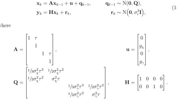
Important properties of SSMs are stochasticity and decoupling of the system dynamics and measurements. As an example, the target tracking state must contain at least the target's location and velocity. SSMs are a general framework and in any specific application prior knowledge of the system must be brought in.
The mathematical form of the dependence between the measurements and the state must be formulated, as well as the dependence of the state on its predecessors. Depending on the method, this requires either the filtering or the filtering and smoothing solutions of the state estimation problem.

State space models
The sensitivity of the posterior marginal distribution to the prior depends on the amount of data (the more data the less sensitivity). The measurement model p(yk|xk,θ) models how observations depend on state and noise statistics. In terms of notation, we will superimpose p(· | ·) as a generic probability density function specified by its arguments.
This means that fk and hk and the PDFs of qk−1 and rk will be independent of k. It is clear that the maps f :X → X and h:X → Y in equation (5) indicate the mean values. of the dynamic and measurement models:.
Bayesian optimal filtering and smoothing
Kalman filter
The Kalman filter is the most well-known filter, first introduced in the seminal article by Kalman (1960). With the help of Lemmas A.1 and A.2, the derivation of the Kalman filter equations is quite simple (Särkkä, 2006). 21g) This includes sufficient statistics for joint T distributions.
Rauch–Tung–Striebel Smoother
Nonlinear-Gaussian SSMs
- Gaussian filtering and smoothing
- Numerical integration approach
- Cubature Kalman Filter and Smoother
- Maximum a posteriori and maximum likelihood
- Ascent methods
Assume that the smoothing distribution of the previous step, p(xk+1|y1:T), is available. For static parameters, the part of the dynamic model corresponding to the parameters is set to identity. Classically, an extended Kalman filter is then used to approximate the probability distribution of the augmented state vector in the joint parameter and state space.
In the Bayesian sense, the complete answer to the filtering and parameter estimation problems would be the joint posterior distribution of the states and the parameters. If the support of the prior then includes the true parameter value, the MAP estimate has the same asymptotic properties as the ML estimate (Cappé et al., 2005).
Gradient based nonlinear optimization
Linear-Gaussian SSMs
Let us next focus on computing the gradient of the log-likelihoodℓ(θ) function, also known as thescore function. By marginalizing the joint distribution of equation (22) we get 61) Applying equation (17) and taking the logarithm then gives C, (62) where C is a constant that does not depend on θ and thus can be ignored in the maximization.
As will be demonstrated shortly, this leads to some additional recursive formulas, known as the sensitivity equations, which allow the gradient to be computed in parallel with the Kalman filter. The second method requires the smooth distributions with the cross-time step covariances and this can be easily computed with the expectation maximization machinery that will be introduced later. When applied to linear-Gaussian SSMs, these two methods can be proven to calculate exactly the same quantity (Cappé et al., 2005).
Here we will also assume that it is independent of θ, since in practice this is often the case (ie, the linear mapping from state to measurement is known). As mentioned earlier, these equations are sometimes known as sensitivity equations and they are derived at least in Gupta and Mehra (1974).
Nonlinear-Gaussian SSMs
Assume that at the current iteration k we have available the approximate mean and variance of the prior filtering distribution, mk−1|k−1 and Pk−1|k−1, as well as the partial derivatives ∂mk−1|k −1∂θ.
Expectation maximization (EM)
Partial E and M steps
Linear-Gaussian SSMs
111) It is then clear that in the E-step one has to calculate the T + 1 smooth distributions, including the T cross-time step distributions, since these will be needed in the expectations. 113) This was a consequence of assuming the Gaussian prior distribution of Equation (5c). Then by applying the manipulation. 117) It is easy to see that the extreme of the last line with respect to A is obtained by setting The next task is to derive the M-step maximization equations for the process and measurement model noise covariance matrices Q and R .
As can be seen from (108), the terms involving Q or R are similar in form, so the resulting maximization equations are analogous. In short, the E-step of the EM algorithm in linear-Gaussian SSMs consists of computing the joint distributions T of equation (114) with the RTS smoother.
Nonlinear-Gaussian SSMs
Our strategy will be to use Gaussian filtering and smoothing in the E-step to compute the expected sufficient statistics. We will settle for an incremental M-step, where we will again use the gradient-based optimization method. This leads to the requirement to be able to calculate ∇θQ(θ,θ′), i.e. the gradient of the intermediate quantity with respect to θ.
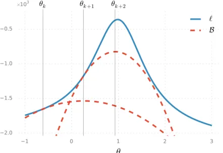
It is quite unclear how many iterations of the optimization algorithm should be performed in the M-step since, as pointed out in section 4.3.1, any new parameter value that increases the log-equity is sufficient. In Lange (1995) a heuristic argument was used to perform only a single iteration of Newton's method in the M step. An obvious strategy is therefore to use a Gaussian smoother to compute the joint smoothing distributions and then compute the 2T expectation integrals by applying the same integration rule as used by the smoother.
To use gradient-based nonlinear optimization in the M step, we need the analytic gradient of the objective function. It is important to highlight at this point that the joint smoothing distribution approximation of equation (126) depends on θ′ (the current, e.g. given, parameter value) and during the M step we search for the next parameter valueθ′′ = arg maxθQ (θ,θ'). Let us then find the formal differential for a general log-Gaussian, where both the mean and the variance depend on the scalar parameter θ.
To assemble the necessary computations evaluateQ(θ,θ′)and∇θQ(θ,θ′) given the sufficient statistics for the T-joint smoothing distributions, let us introduce the shorthand notation fk∇−1,i ≡ ∂f( xk−1 ,θ).
Score computation
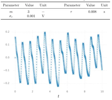
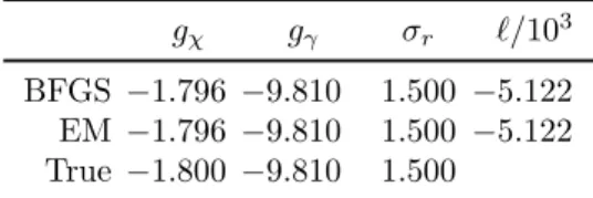
We acquire a series of distance measurements with a radar, so that our data consists of the noisy two-dimensional locations of the object as measured at time points {tk}Tk=1. Let us then proceed to estimate some of the parameters using the noisy measurements as inputs to the two parameter estimation methods we have considered. To inspect the effect of the initial guess as well as that of the specific measurement dataset, we run ranM = 100 simulations with the initial estimate for each parameter θi chosen from the uniform distribution U[0,2θi∗], where θi∗ is the true generative value for parameter i given in Table 1.
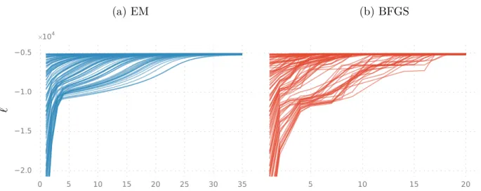
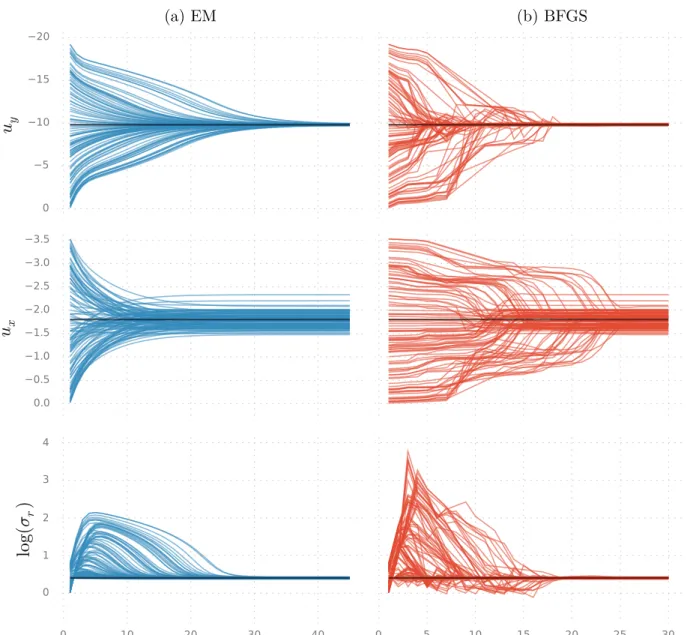
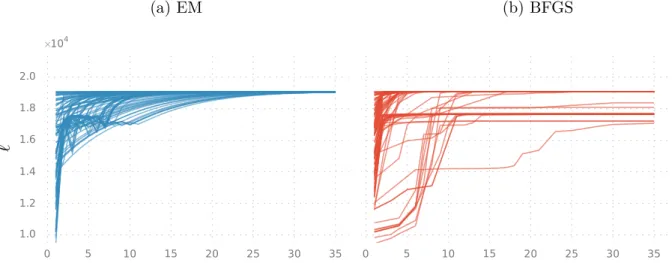
The lengths of the simulated measurement data sets were approximately N ≈1400 with some variance caused by always stopping the simulation when γk < 0 for some k. For each simulated data set and its initial estimate, we ran the EM and the BFGS parameter estimation methods for a joint estimate of the three parameters. In each panel, one line is plotted for each simulated data set and the panels display their quantities as a function of the iteration number of the estimation method.
The convergence profiles show great variation between the methods and between the parameters, but the means of the converged estimates seem in all cases to agree very well with the generative values. In any case, according to the asymptotic theory, the variance of the ML/MAP estimates should go to zero as the amount of data approaches infinity. The fact that the results differ after the sixth decimal point can be explained by different numerical properties of the two algorithms.
Because we use unbiased estimates, the estimation error can be reduced to the size of the machine epsilon by simulating more data points. In conclusion, it appears that in this case the estimation problem was too simple to cause noticeable differences in the performance of the parameter estimation methods. Note that the objective functions of the optimization methods differ in their computational complexity, implying that the graphs cannot be compared directly on the x-axis.
Photoplethysmograph waveform analysis
Our goal now is to find the ML estimate (or, equivalently, the MAP estimate with a uniform prior) of the parameter θP ≡ {σω, σx} using both the gradient-based nonlinear optimization approach presented in Section 4.2.2 as well as the EM approach presented in Section 4.3.3. We will cover the rest of the parameters as recorded with the values presented in Table 3. As with the analysis of the ballistic projectile in Section 5.1, the BFGS implementation used was the fminunc function included in the Matlab Optimization Toolbox.
Contrary to the linear SSM analyzed in the previous section, we can see here that the convergence of EM is not monotonic in all cases. The first thing to note is the big difference in the behavior of the methods. For better insight into the behavior of the parameter estimation methods, illustrate the convergence of ℓ as a function of the logarithms of σω and σx.
It appears that there are small local maxima on either side of the large local maximum around logσx ≈ −3. Some of the BFGS optimization runs (31 out of 100 to be specific) converge to the small local maxima. Note that the objective functions of the optimization methods differ in their computational complexity, implying that the graphs cannot be compared directly on the x-axis.
Since the static parameter estimation problem is closely related to filtering and smoothing problems, the focus of the first part of the thesis was on state estimation. The main appeal of gradient-based nonlinear optimization methods is their order of convergence, which can be quadratic. Thus, some of the strengths and weaknesses that were mentioned in the previous chapter when comparing sensitivity equations and Fisher's identity apply directly when comparing sensitivity equations with the EM solution.
The disparity in the approximations appears to be demonstrated in the results of the two demonstrations in Section 5. Models and Algorithms for Tracking Maneuvering Objects Using Variable Velocity Particle Filters. Proceedings of the IEEE.