at Earth and Mars

The original idea of the new analysis approach for the Mars Express radio occultation data was formulated by Dr P.-L. The work presented in this thesis focuses on the ionospheres of Earth and Mars and their behaviors in response to the direction of the solar wind.

Neutral atmospheres

Above 100 km altitude, that is in the thermosphere, the influence of the 11-year solar cycle is significant. Height profiles of the Martian atmosphere at the time of landing and location of the Curiosity rover, provided by the Mars Climate Database v5.2.

Figure 1.1. Altitude profiles in the terrestrial atmosphere above Sodankyl¨a on 1 January 2014 at 12:00 local time, taken from the MSIS-90 model

Ionospheres

Photoionisation, chemistry and transport

Because the ion movement is not in the same direction as the electron movement, currents flow in the plasma. Ambipolar diffusion of electrons and ions, mainly upward, also plays a role in the field-directed movement of charged particles [Rees, 1989].

Structures of the terrestrial and Martian ionospheres 7

Typical electron density profiles in the daytime (black, solid) and nighttime (black, dashed) terrestrial ionosphere (after Cravens [1997]). Density profiles of the main ion species in the diurnal ionosphere are given in color.

Figure 1.3. Typical electron density profiles in the daytime (black, solid) and nighttime (black, dashed) terrestrial ionosphere (after Cravens [1997])

General properties

In the case of the Earth, for example, there is a strong coupling between the ionosphere, the magnetosphere (described in section 1.3.1) and the solar wind. The most extreme type of disturbance occurs when solar plasma is released from the surface of the Sun, forming a so-called coronal mass ejection (CME).

High-speed streams

Main solar wind parameters measured near Earth during a high-speed stream event from March 2007. From top to bottom: IMF magnitude, solar wind velocity, solar wind density and solar wind dynamic pressure.

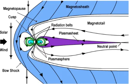
Magnetospheres

Terrestrial magnetosphere

They correspond to holes in the Earth's magnetic shield through which the solar wind can directly enter the geomagnetic cavity. Schematic diagram of the Martian induced magnetosphere. reproduced fromBrain et al.[2017]; courtesy of Fran Bagenal and Steve Bartlett).

Martian induced magnetosphere

However, interactions of the Martian environment with the incoming solar wind result in the formation of an induced magnetosphere. Because the Martian dayside ionosphere is dense enough (see Figure 1.4), it acts as a barrier to the solar wind as a conducting medium. As the name suggests, this boundary also represents the boundary of the magnetic accretion region, where the magnetic field lines of the solar wind are wrapped around the Martian ionosphere and stretched into a magnetic tail-like structure.

The draping takes place in or close to the plane containing the solar wind speed and IMF vectors as seen from Mars [Crider et al., 2004]. The polarity of the tail lobes is determined by the IMF component perpendicular to the speed of the solar wind. In the central part of the tail, heavy ions (primarily O+ ions) are accelerated from 0.1 to a few keV through energy transfer from the magnetic field of the solar wind to the Martian plasma [Nagy et al., 2004].

Planetary environments and solar wind interactions

Reconnection and convection
Geomagnetic storms and magnetospheric substorms
Particle precipitation
Some aspects of Mars interactions with the solar wind
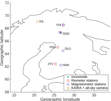
Sodankyl¨a ionosonde
IMAGE magnetometers
SGO riometer chain and KAIRA
Kilpisj¨arvi All-Sky Camera

As the magnetic field builds up in the magnetic tail (5), it compresses in the vicinity of the neutral sheet. Auroral emissions on Earth are often studied at three wavelengths in the visible part of the electromagnetic spectrum. This type of aurora is especially common during the morning hours in the equatorial part of the auroral oval [Kvifte and Pettersen, 1969].

Ionosondes (ionosphere probes) are radar systems designed to measure parameters related to the electron density profile in the ionosphere. The critical frequencies of the O mode are directly related to the density of electron peaks in the ionospheric layers. The strength of the radio signal observed by the rheometer therefore depends on the distribution of the radio sources in

Figure 1.8. Magnetospheric and polar cap convection driven by magnetic reconnec- reconnec-tion with southward IMF

Satellites

Mars Express

Each camera image contains 512×512 pixels and, when projected at 100 km altitude, corresponds to a field of view approximately 600 km in diameter. In Paper III, a pulsating aurora event is studied with optical data from the Kilpisj¨arvi all-sky camera.

NOAA/POES

ACE

Superposed epoch analysis

Classical version

A critical aspect in nested epoch analysis is the choice of zero epochs. 2008] have shown that, depending on the chosen criterion for defining the zero epochs, different features can be more or less prominent in the response of the studied parameters of the system. This implies that the selection of the zero epoch must be adapted to the physical constraints associated with the studied parameters.

Phase-locked version

Comparison of standard (left panels) and phase-locked (right panels) versions of the superimposed epoch method. upper panels). Time series representing 30 events following noisy cosine functions, amplified strength >0. lower panels) Mean values of the time series calculated using the nested epoch method. Panel (a) shows the time series of the 30 signals and panel (c) shows the mean values obtained by the classical nested epoch method.

The visible features in the mean curve are essentially noisy, and the effect of the ramp function after the zero epoch is not clearly displayed. In the phase-locked version of nested epoch analysis, the time series corresponding to each event are shifted in time such that they are all in phase. As a result, the curve corresponding to their mean values, shown in panel (d), is very close to an amplified cosine function at t > 0, thus revealing the effect of the ramp function after the zero epoch.

Figure 3.1. Comparison of the standard (left panels) and phase-locked (right panels) versions of the superposed epoch method

Radio-occultation

Principle
Data analysis
Solar wind driving
Overview of ionospheric response to high-speed streams
E and F region responses
Energetic particle precipitation

Sharp increases in IMF size were detected by calculating the time derivative of IMF power using a central difference scheme (criterion (i)). Each high-velocity streaming event candidate was then validated by a visual inspection of the behaviors of the solar wind parameters, and some spurious events were removed during this process. However, Paper I does not address the possible effects of transport, which is likely to play an important role in the dynamics of the F region.

This increased activity may be due to the annual variation of the Earth's magnetic dipole direction [Russell and McPherron, 1973]. Cosmic noise absorption is generally produced by energetic (>30 keV) particle precipitation, which ionizes the D region of the ionosphere. The MLT distributions of these three types of CNA events at each of the four riometer stations used in the study are shown in Figure 4.4.

Figure 3.3. Overview of the radio-occultation model (colourised version of Figure 1 from Paper IV).

Modulation of energetic precipitation during pulsating aurora

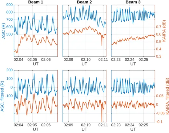
To assess whether the CNA modulations could originate from electron density variations in the lower region where optical emissions come from (~100 km altitude), simulations are performed using the Sodankyl¨a Ion-Neutral Chemistry (SIC) model [Verronen et al. ., 2005]. SIC is a one-dimensional coupled chemistry model of the middle atmosphere which includes the solution of the continuity equation for ions and neutral species in the D region, taking into account production processes including extreme solar ultraviolet and X-ray radiation, particle precipitation and galactic cosmic rays, and loss processes through multiple hundred reactions. In the first scenario, the deposition spectrum is modulated (5 s on, 5 s off sequences, 25% modulation, based on beam 1 observations) only for energies up to 10 keV, i.e. auroral energies that reach down to about 100 km height in the ionosphere.

In the second scenario, the modulation is applied to all energies in the precipitation spectrum, i.e. including energies which affect the D region. The results presented in Paper III may help to understand the mechanism behind the origin of pulsating auroras. These results lend support to a model proposed by Miyoshi et al b] in which chorus waves propagating along the field line can cause broad-energy electron loss cone scattering simultaneously, thus predicting that electron precipitation is modulated over a wide energy range during pulsating auroras.

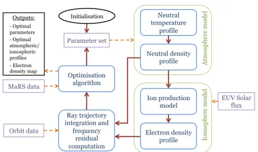
Figure 4.5. Time series of the data during pulsating time intervals in beams number 1, 2 and 3

Analysis of Mars Express data with the radio-occultation model

Reproduction of the frequency residual profile

The results show that the CNA modulation resulting from the first scenario is one order of magnitude too low in amplitude compared to what is observed in beam 1, while the second scenario leads to CNA pulsations with amplitudes close to those observed. This altitude range corresponds to the lower ionosphere, and a possible reason for this difference may be related to the X-ray and UV components of the solar flux model used as input. While in the ionosphere the main M2 electron density peak is well reproduced, the M1 layer model is overestimated.

This corresponds to the height range where the frequency residual is also not well reproduced, indicating that both problems may have the same origin. At lower altitudes, in the neutral atmosphere, the comparison of neutral density profiles obtained with both methods shows good agreement. However, significant differences can be seen in the temperature profiles, not only near the heights where a boundary condition is needed for the classical inversion, but also down to the ground.

Figure 4.6. Frequency residual profiles for the experiment of 28 April 2007. The thick black line shows the MaRS measurements, and the grey line shows the frequency residual simulated by the model

Influence of medium asymmetry

Due to the ellipticity of the Martian orbit, the angles are shown when Mars is at its perihelion (blue) and aphelion (red). The dashed-black line shows the trajectory of the lowest beam before occultation, thus defining the boundary of the domain where radio waves propagate during the occultation experiment. Ionospheric density profiles, showing simulated electron (red), O+2 (dashed blue), O+ (solid blue), CO+2 (purple) and NO+ (green) number densities, and electron density (dark blue) obtained with the radioscience classic inversion.

Figure 4.7. (left) Sketch of the Sun–Earth–Mars configuration indicating the possible locations of the occultation point during a radio-occultation experiment, seen in the ecliptic plane

Ion density profiles

The overall agreement between these two profiles is quite good, especially near the main peak (M2). However, discrepancies are visible above the peak, where the modeled electron densities are lower than those obtained with the classical inversion method. This may be due to the fact that the current version of the ionospheric model used in the radio occultation data analysis method does not include effects of vertical species transport.

Another discrepancy can be seen near the peak of the secondary electron density (M1), where the model also gives lower electron densities compared to the classical inversion. Understanding the origin of this difference still requires future work; this may be related to the fact that the X-ray and EUV components of the solar irradiance spectrum are subject to significant variability.

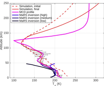
Improvements introduced in Paper V

Comparison of the initial (dashed red line) and final (solid red line, with error bars) atmospheric temperature profile for the experiment on 28 April 2007. The scarlet line shows the neutral temperature profile given by the Mars Climate Database (MCD) v5. 2 for the conditions of the experiment. The new approach is based on direct simulations of radio wave propagation in the Martian atmosphere and ionosphere during a radio occultation experiment.

This upgrade of the model improved the overall analysis of the Mars Express radio occultation data. Jakosky (2015), The first in situ electron temperature and density measurements of the Martian nightside ionosphere, Geophys. Boehm (1994), The ionospheric signature of the cusp: A case study using Freja and the Sondrestrom radar, Geophys.

McPherron (1973), Semiannual variation of geomagnetic activity, J. 1852), on periodic laws discoverable in the average effects of larger magnetic disturbances. Tsybulya (2013), Global model of the peak height of the F2 layer for low solar activity based on GPS radio occultation data, J.