Classical methods for solving PDE models
Introduction
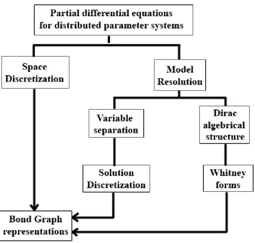
The exchange of energy and information between components can be presented in a graphical way, which contains everything necessary to obtain the dynamic evolution of the model. There are two classes of approximation: equation approximation (finite difference volumes) and solution approximation (variation methods, finite element methods).
Partial differential equations
The variational methods such as Galerkin, Rayleigh-Ritz and least squares differ from each other in the choice of integral form, weight function and/or approximation functions. Partial differential equations (PDE) are classified according to their order, boundary condition type, and degree of linearity (yes, no, or quasi).
Solving PDE
- The method of weighted residual
- The method of separation of variables
- Spectral methods
- Finite element method
- Finite difference method
- Finite volume method
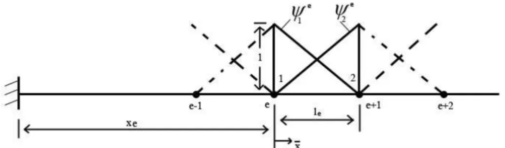
This is a representation in terms of the global coordinate x (i.e., the coordinate of the problem) and only for an element domain Ωe. The basic idea of the finite difference method is to replace derivatives with finite differences.
Conclusion
To solve a problem with the variable separation method, Karnopp and allen [KAR 90] proposed to split the domain into a sufficient number of modes and replace the neglected others with an equivalent stiffness to reduce the static character of the system not to lose. Spectral methods generate algebraic equations with full matrices, but to compensate, the high order of the basis functions gives high accuracy for a given N. However, they are most useful when the geometry of the problem is fairly smooth and regular.
Port-Hamiltonian systems
Introduction
The elements interact with the environment through the gates, and the product between the input and output signals is represented by the instantaneous power. The power exchange between components and between the system and its environment can be represented mathematically by a Dirac structure in the case of finite dimensions or by a Stokes-Dirac structure in an infinite dimension, the most important property of which is its conservativeness. The dynamics of the model is specified when an energy function (Hamiltonian) and the space of energy variables are defined.
The principle of least action
In this chapter we will make a presentation of the formalism, and then through an application we will present the extension of telegraph equations in the infinite dimensional case with dissipation [Che 07], [Che 09]. The actual trajectory of the particle must have δS =0 (Appendix 1) and thus satisfy the Euler-Lagrange equations. In general, if the system has n degrees of freedom, q1,..,qn, are the Lagrange's equations of motion.
Hamiltonian formalism
- Port Hamiltonian representation
This concept is used in the representation of the system as a net connecting components [Sch 02]. Denote by Λ Ωk( ) the vector space for k-forms on Ω and by Λ ∂Ωk( ) the vector space for k-forms on the boundary. The port-Hamiltonian system with dissipation defined in terms of the Dirac structure satisfies the power inequality: .
Transmission line application
- Without dissipation
- With dissipation
- Spatial discretization
- Constitutive equations
To introduce the energy variables, we write the transmission line power balance starting with the total energy. The last two terms of the left side of equation (2.70) represent the power flow at the boundary and the power dissipation in a transmission line. The electrical layout of the transmission line at the element level is shown in the following figure.
Conclusion
Thus, the entire transmission line can be reconstructed by connecting a fixed number of cells in advance.
Traffic flow models
Introduction
In the context of economic globalization, the need to circulate goods and people has experienced a new growth. All of these theories lead to models and tools used in the design and operation of streets and highways. The first study of traffic flow was done in the 1930s using probability theory to describe road traffic by Adams [Ada 36].
Model classification
In this chapter we present a classification of the models used in the representation of traffic flows, followed by a brief presentation of the main schemes used in numerical simulation, and some results. We can therefore have continuous models or discrete models depending on when changes occur in the state of the traffic system. In the suite we will give a short presentation of the microscopic and mesoscopic models, then we will present the macroscopic models that are of interest to us.
Microscopic and mesoscopic models
When we want to simulate the flow of traffic, we must be aware that we have different conditions when we talk about a simulation of a highway or an entire city. Mesoscopic flow models describe the separation of vehicles in a general term using example probability distribution functions. The most popular models used to model traffic flow at this level of detail are the forward distribution models developed by Buckley [Buc 68], Branston [Bra 76], Hoogendoorn and Bovy [Hoo 98], the cluster models developed by Prigogine [Pri 61], Prigogine and Herman [Pri 71], Botma [Bot 78] and gas-kinetic continuum models developed by Prigogine and Herman [Pri 71], Paveri-Fontana [Pav 75], Nelson [Nel 95] , Helbing [Hel 97], Klar and Wegener [Kla 98], Hoogendoorn and Bovy [Hoo 00].
Macroscopic models
He extended the LWR model with a partial differential equation that describes the dynamics of the velocity v. The merging problem has been studied by Daganzo [Day 95], Holden and Risebro [Hol 95] and Lebacque [Leb 96]. The supply” is the flow rate when the traffic situation is too critical and the cell flow capacity when it is subcritical; "the.
Numerical methods
To solve the boundary problem, they used either the solution of the Riemann problem at the boundary or the supply-demand method where it calculates the supply and the demand for each cell, and then selects the minimum between them as the boundary flow. So, what needs to be done is to ensure o distribution of the flow for all the current cells. The characteristics of the initial state are diverse, so we have a number of solutions, and the physical one is selected using the entropy criterion, which in the traffic flow corresponds to a series of characteristics (fig. 3.4).
Implementation
- Riemann problem in the LWR model
- Influence of the choice of a numerical method
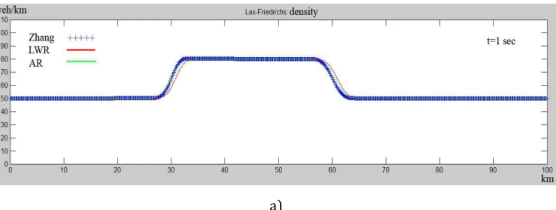
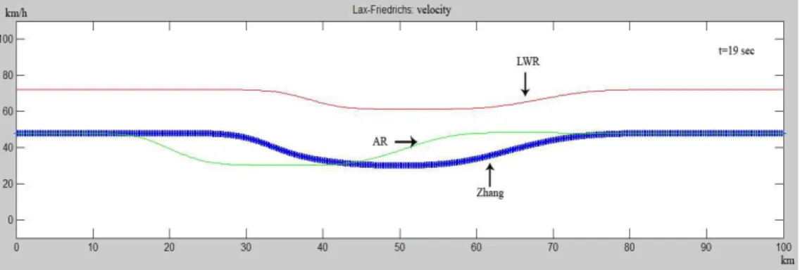
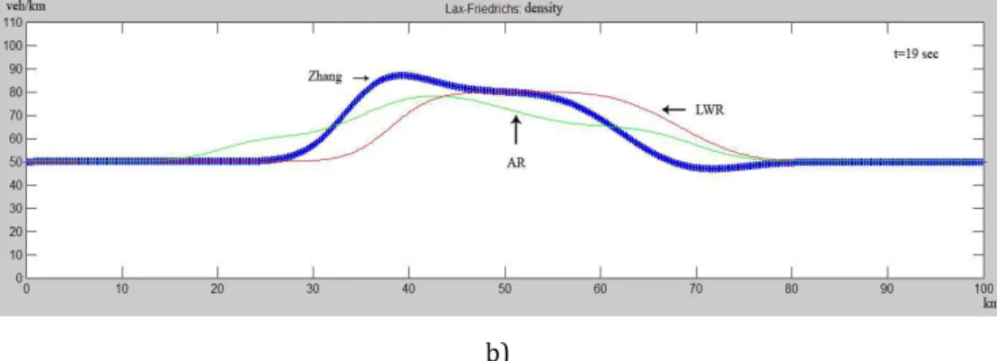
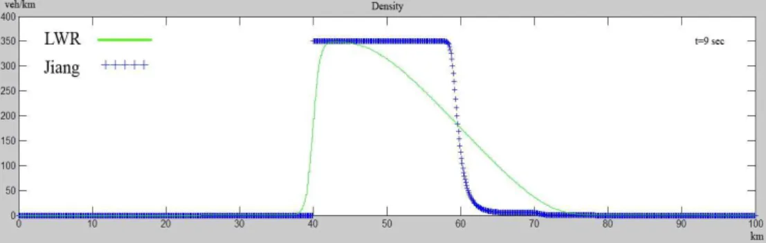
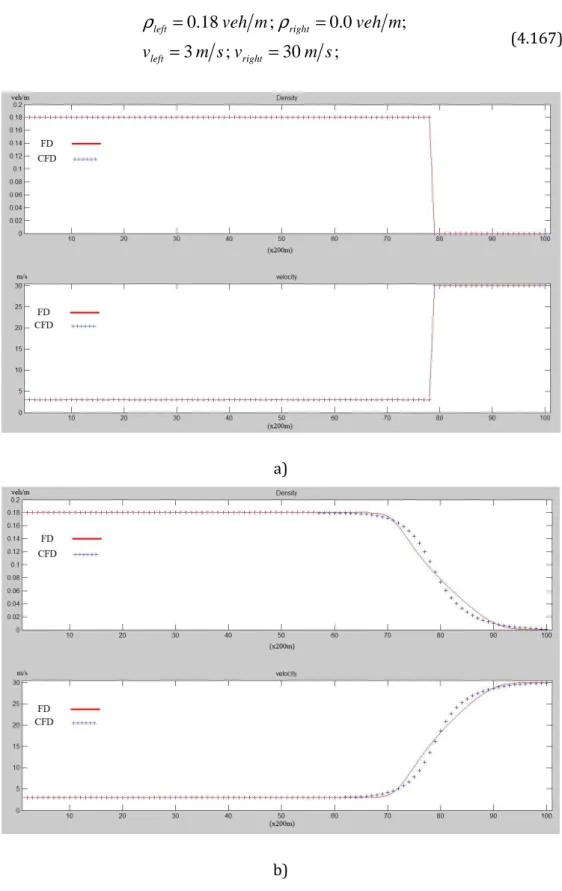
The Jiang model seems to give better results on the back side of the front. In both cases we have almost the same shape for density and velocity with a small bump at the rear of the front in the CFD approach. A port Hamilton system was used to represent distributed parameter systems.
Comparison of LWR and Jiang models
Consider the LWR model discretized using the Lax-Friedrichs scheme and the model proposed by Jiang [Jia 02]. This model was discretized by [Jia 02] using the following scheme: for density and for velocity: . 3.49). At the velocity level, there is an algebraic relationship to density in the LWR model.
Conclusions
The LWR model is a model that has long been used in simulations and has been considered the best model to represent traffic flow. By simulating the models found in the literature, we saw the advantages and disadvantages of each of them. In the meantime, we tried to find out which numerical method (based on the finite difference) is more appropriate to use in the discretization of the models.
Transport equations modeled by CFD
Introduction
- Two-equation traffic models
To address these shortcomings, a new type of model has been proposed that considers two dynamic equations, one for vehicle density and one for vehicle speed. Recent years have seen the development of CFDs using the bond graph approach [Bal 06]. Two-equation traffic models consider a one-dimensional flow with one continuity equation for the vehicle density ρ( )x t,.
Power balance per unit volume
- Kinetic energy
- Balance equations
Starting from this approach, in this chapter we will present a new way of modeling traffic flow using computational fluid dynamics. The balance equations are the power density equations corresponding to each of the terms that contribute to the time derivative of the total energy density.
Discretization
- Description of the flow fields
- Integrated variables
The representation of the flow fields in terms of nodal values and interpolation functions allows to define the corresponding values at any position, so that it is possible to uniquely calculate all the integrals corresponding to the equations of state; this is not clear for other methodologies such as finite differences or finite volumes, where only nodal values are defined and additional considerations must be made to integrate the differential equations. Moreover, the chosen representation can make use of the considerable amount of computational tools already available for the popular Finite Element Method.
System integration
- Kinetic energy
- System IC -field
- Resistance field
Modulating transformer connecting the nodal vectors of vehicle speed and torque. 4.25), the nodal vector of the vehicle moment can be considered as an integral system of local values weighted by the speed interpolation function. It can be easily shown that the vehicle momentum of the system Q can be obtained as:. 4.24), the knot vector K can be considered as an average of the domain of the system of the corresponding local values, weighted by the interpolation functions. It can also be shown that the volume integrals of the right-hand side term of Eq.

State equations
- Mass port
- Velocity port
By making the product of K times Eq.(4.43) it can be easily shown that the integral density balance equation is satisfied, which is: Adding the node components of Eq. 4.50) it can be easily shown that the integral rate equation is satisfied, i.e. Making the product of Eq. 4.50) times v it can be easily shown that the integral velocity balance equation is satisfied, which is:
Coupling matrices
- Coupling between the velocity and mass ports
Since the interpolation function was chosen as the test functions, the product FXT.v, where FX is any nodal force vector, recovers the corresponding power term integrated into the system.
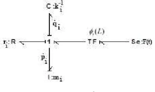
System Bond Graph
Initial and boundary conditions
- Initial conditions
- Boundary conditions
Boundary conditions establish relationships between variables corresponding to nodes located at the boundary of the system and can be considered (in the linkage graph methodology) as input variables. It is necessary, for the model to be mathematically well defined, that the boundary conditions allow causality to be determined for all links in the resulting link graph. Boundary conditions are introduced through the couplings corresponding to the surface source terms mɺ( )BΓ.
Integrated variables
- Shape and weight functions
- Diagonal volume matrix
- Nodal vector of mass
- Inertia matrix
- Nodal vectors of potentials
- State equations, mass port
- State equations, velocity port
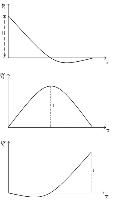
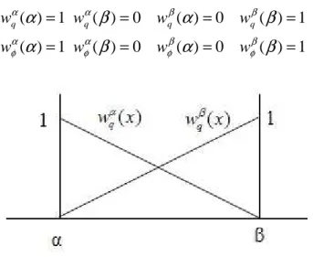
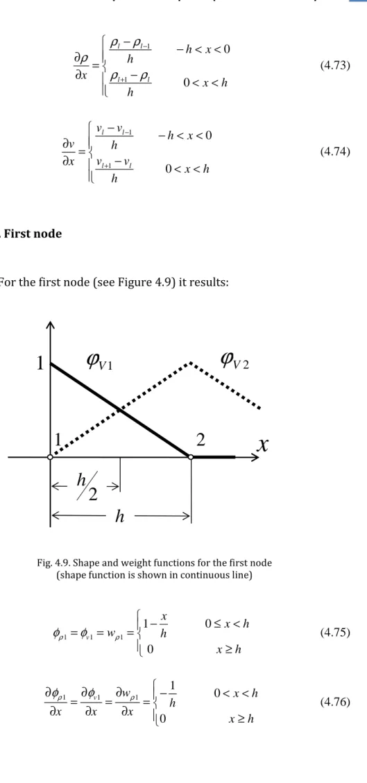
Shape and weight functions for an interior node (shape function is shown in solid line). Shape and weight functions for the first node (shape function is shown in solid line). Shape and weight functions for the last node (shape function is shown in solid line).
Implementation
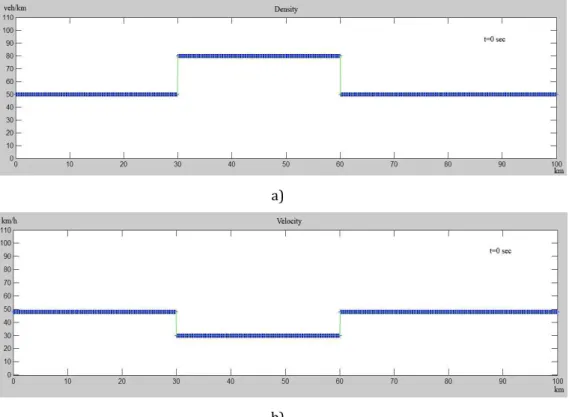
We consider the rarefaction wave, which appears in the case of a stop and go situation (red color) with the initial conditions shown in figure 4.11. a). When we have a queue of vehicles that produce a shock wave at the rear, with the initial conditions shown in figure 4.12.a), after 40 seconds we get the graph from figure 4.12.b). A smaller Δt will define a smaller diffusive collision at the rear of the front and a speed smaller than the propagation speed of the shock wave.
Conclusions
Elements of a kinetic theory of traffic flow”, Proceedings of the Eleventh International Symposium on Rarefied Gas Dynamics, Vol.1, Cannes, France, pp.129-138. A mathematical model of traffic flow in a one-way road network”, SIAM Journal on Mathematical Analysis 26 (4), pp.999–1017. On Boltzmann-like treatments for traffic flow: a critical review of the basic model and an alternative proposal for diluted traffic analysis', Transportation Research B 9, pp.225-235.