Concluding remarks on the findings as well as policy recommendations are presented in the last section. Applications of this new growth theory to environmental issues began in the 1990s with Nordhaus (1999), Goulder and Schneider (1999), Goulder and Mathai (2000), Buonanno et al. Our dynamical framework has a representative family with infinite lives, as in the Ramsey (1928) model, and introduces population growth in the Romer (1990) R&D model.
All prices in the model are in relative terms, and the wage rate is the numeraire in the model. This means that the scarcity rent (i.e. the value of granted permits) is also integrated into the price limit at the lowest level of the production structure. The endogenous growth framework based on Romer (1990) assumes an increase in the productivity of all inputs. The development mechanism includes three assumptions: 1) technological change causes growth, 2) the market values that result in innovations, and 3) knowledge serves as a non-rival input in the research sector.
The market price Pmon is equal to the marginal cost of production adjusted according to the elasticity of demand for development goods in the final goods sector: Pmon = Piv σKE). Market power in the monopolistic development sector forces the private optimum to deviate from the social optimum. Production technology in the development sector is similar to the input-output structure in high-tech sectors (NIS, 2006a).
Its production cost calibration is consistent with the principles of production in the final goods sector, and the sector's monopoly price is obtained by summing the monopoly rent.
Simulations and discussion
Prices versus quantities in an endogenous growth approach
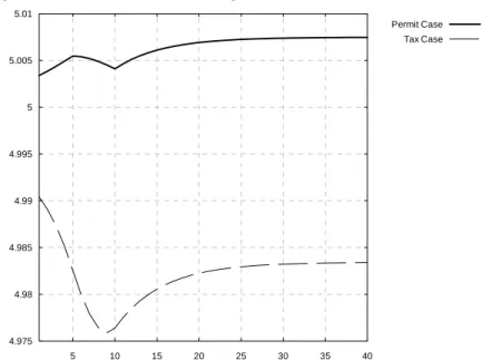
In the leave scenario, households anticipate an increase in the aggregate price of consumption during the shock, as well as a decrease in this price after 2012; thus, consumption follows an opposite evolution. The evolution is different in the tax scenario, as paying carbon taxes offers less investment opportunities for agents. Flexibility is enhanced in the latter case by the fact that the initial allocation of permissions is grandfathered.
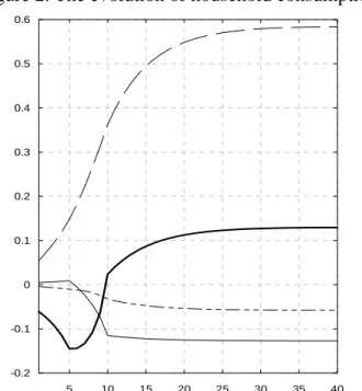
At household level, welfare falls in the permit case (-0.13%) and improves in the tax scenario (0.58%). This result can also be quite surprising compared to the permit scenario, because the variation in consumption is positive in the terminal period. Rather, the counterintuitive finding that welfare improves under a tax scenario but falls in the permit scenario is explained by shifts in the key indicators that comprise welfare.
For example, in the permission scenario, individuals expect a decrease in the long-run aggregate price and make a trade-off that favors long-run consumption. The variation in household income tends to zero in the permit scenario but increases in the tax scenario, mainly due to variations in social transfers. Intertemporal household income also increases in the tax scenario because the discount rate that values individual income is lowered.
The differentiation in interest rate variations between the two scenarios shows divergent growth trajectories: the expanded growth in the permit scenario requires more investment (0.29%) compared to the tax scenario (-0.07%), which implies a different evolutionary trajectory for the rate of the discount. . A decrease in the interest rate in the tax scenarios implies a greater decrease in the savings of individuals (-0.8%) than in the leave scenario (-0.5%); This effect is reinforced by the deflationary impact of the policy, as consumption is encouraged at the expense of saving. If consumption is used as a welfare measure, both policies would show positive effects in the final simulation period.
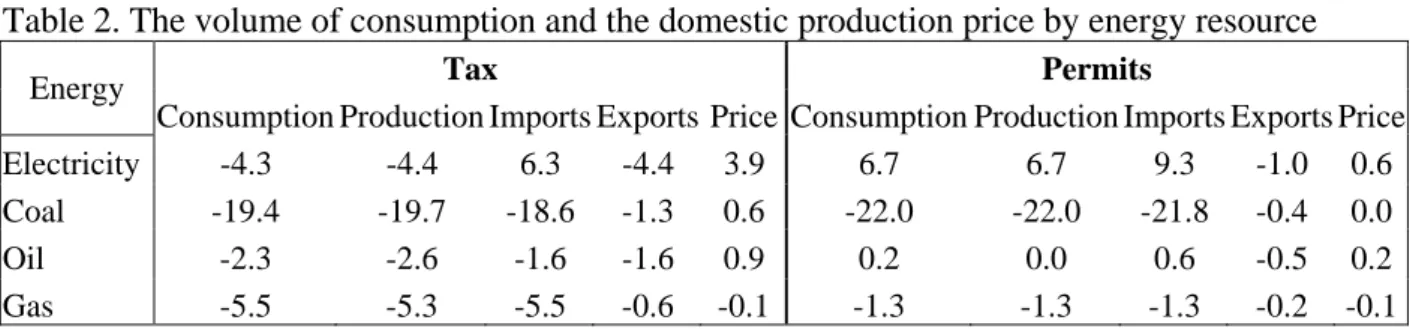
But this indicator does not take into account the transitory impacts of the policy, such as the drop in consumption before the shock in the permits scenario. In the tax scenario, the country's energy dependence is reduced due to contractions in productive activities. Regarding the import structure, an increase in the volume of electricity is observed, but the country does not lose its status as a net exporter of electricity.
Endogenous versus exogenous growth
This is because the same environmental constraints actually represent stricter constraints in the exogenous growth scenario compared to the endogenous growth scenario, as no spillovers are generated. In the tax scenario, welfare varies positively with growth in both cases, albeit in a larger percentage with endogenous growth. The capital volume is higher under endogenous growth in the permit market scenario, but lower under endogenous growth in the tax scenario.
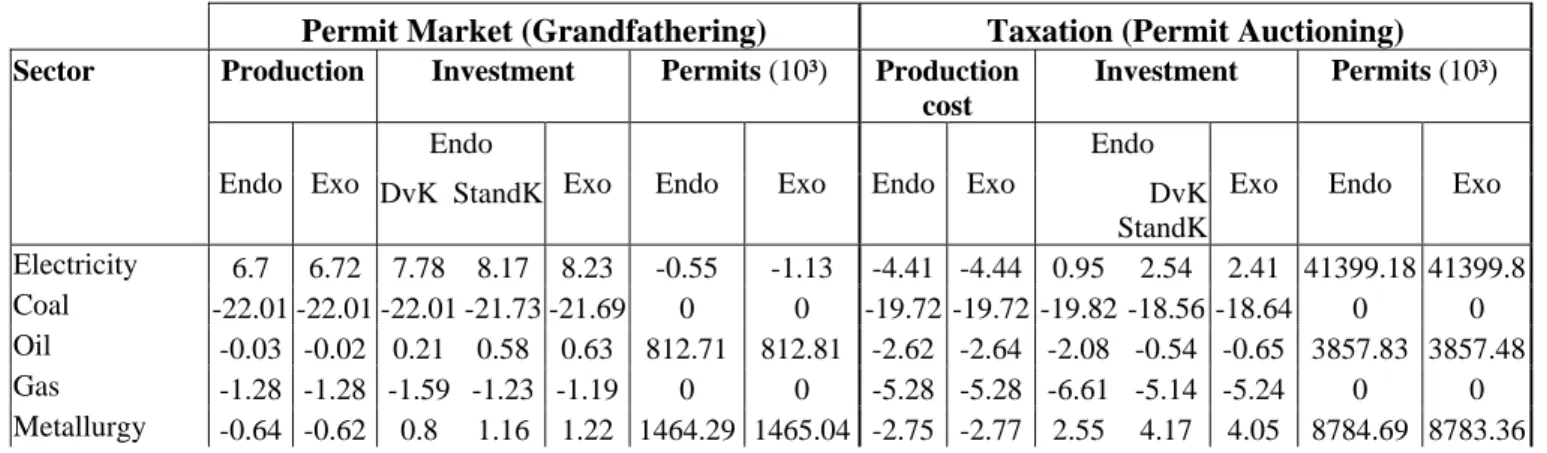
In the permit scenario, investments increase with respect to both development and standard capital goods. Despite price increases, the demand for development goods improves slightly due to spillover effects generated by positive variations in the growth rate. An opposite effect is seen in the tax scenario, in which the demand for development goods decreases, generating fewer spillover effects.
A higher level of investment in conventional capital reduces investment in research; this is a situation that the literature has described as a "crowding" effect (Nordhaus, 2002). According to the free permit market simulation, demand for development goods increases in sectors such as electricity, refineries, metallurgy, chemicals, and construction, but falls in the remaining sectors. A greater variation in development capital is recorded in the electricity sector, which is the main supplier of energy in the simulated economy.
The analysis focuses here on the qualitative impact of the permit trade during endogenous growth. The amount traded under the exogenous growth scenario is larger compared to endogenous growth. Given the increased activity during exogenous growth, the increase in demand for polluter rights appears justified.
Since endogenous growth provides additional productivity gains and involves fewer structural changes, the permit stock is lowered in all sectors. In contrast, the results under endogenous growth differ depending on whether the policy is announced or not. Thus, the endogenous and exogenous growth versions of our model differ in this perspective, and it appears that the expectations of agents have a more significant impact under the endogenous growth scenario than under exogenous growth.
Conclusions and policy recommendations
However, both policies have a negative impact on the public deficit, which is increasing sharply, indicating that additional financing is needed to ensure the financial health of the Romanian economy. The small difference between endogenous and exogenous growth results is due to the low level of financial and human resources involved in research and development activities in Romania. I am very grateful to Daniel Thery and two anonymous referees, who provided many constructive comments and critical feedback, which led to a significant improvement of the paper.
Bohringer, C., Rutherford, T.F., 1997, "Carbon taxes with exemptions in an open economy: a general equilibrium analysis of the German tax initiative", Journal of Environmental Economics and Management. Goulder, L.H., 2004, Induced Technological Change and Climate Policy, Pew Center on Global Climate Change Report, Washington DC. Goulder, L., Mathai, K., 2000, "Optimal CO2-reduktion i nærvær af induceret teknisk forandring", Journal of Environmental Economics and Management, 39: 1-38.
Goulder, L.A., Schneider, S.H., 1999, “Induced technological change and the attractiveness of carbon reduction policies”, Resource and Energy Economics. European Commission, 2008, 'Proposal for a Directive of the European Parliament and of the Council amending Directive 2003/87/EC to improve and extend the greenhouse gas emission allowance trading system of the Community', COM(2008) 16 final COD), Brussels. European Commission, 2003, Directive 2003/87/EC of the European Parliament and of the Council of 13 October 2003 establishing a scheme for greenhouse gas emission allowance trading within the Community and amending Council Directive 96/61EC.
Kohler, J., Grubb, M., Popp, D., 2006, "Transition to Endogenous Technical Change in Climate Economy Models: A Technical Overview for the Innovation Modeling Benchmark Project", The Energy Journal, Special Issue: Endogenous Technological Change and the Economics of Atmospheric Stabilization: 17-55. Koopmans, T.C., 1965, “On the concept of optimal economic growth”, in The Econometric Approach to Development Planning, Amsterdam. Manne, A.S., Richels, R.G., 2002, “Impact of learning by doing on the timing and costs of CO2 abatement”, Working Paper, Stanford University, CA.
McKibbin, W.J., Wilcoxen, P.J., 1995, "The Theoretical and Empirical Structure of the G-Cubed Model", Discussion Papers 118, Brookings Institution International Economics. Rao, S., Keppo, I., Riahi, K., 2006, "The Importance of Technological Change and Spillovers in Long-Term Climate Policy", The Energy Journal, Special Issue: Endogenous Technological Change and the Economics of Atmospheric Stabilization: 25 - 41. Weyant, J.P., Olavson, T., 1999, "Issues in Modeling Induced Technological Change in Energy, Environmental and Climate Policy", Environmental Modeling and Assessment.
The nested production function
Model equations
TREH - transfers from firms to households TRHE- transfers from households to firms TRES- transfers from firms to government. VAT DDD ACC - value added tax, customs and excise difc- adjustment variable for the state's budget neutrality.
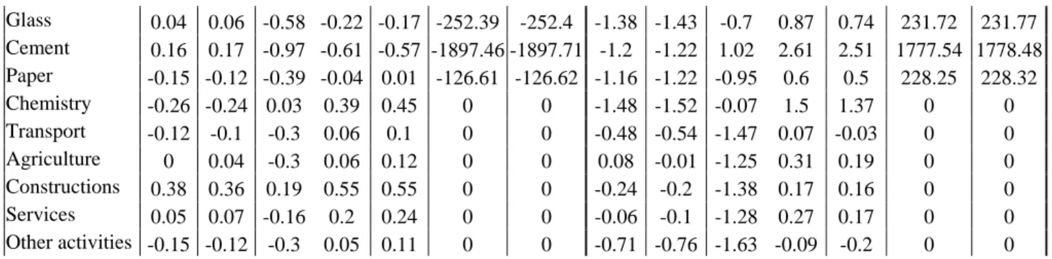
Simulations results (%, reference = 0)