Floorplan Generation from 3D Point Clouds: a space partitioning approach
Hao Fanga,b, Florent Lafargec, Cihui Panb, Hui Huang1a
aShenzhen University
bBeiKe
cUniversit´e Cˆote d’Azur, Inria
Abstract
We propose a novel approach to automatically reconstruct the floorplan of in- door environments from raw sensor data. In contrast to existing methods that generate floorplans under the form of a planar graph by detecting corner points and connecting them, our framework employs a strategy that decomposes the space into a polygonal partition and selects edges that belong to wall struc- tures by energy minimization. By relying on a efficient space-partitioning data structure instead of a traditional and delicate corner detection task, our frame- work offers a high robustness to imperfect data. We demonstrate the potential of our algorithm on both RGBD and LIDAR points scanned from simple to complex scenes. Experimental results indicate that our method is competitive with respect to existing methods in terms of geometric accuracy and output simplicity.
Keywords: Indoor Scene, Point Cloud, Floorplan Reconstruction, Primitive Detection, Integer Programming, Markov Random Field
1. Introduction
Reconstructing the floorplan of indoor scenes from raw 3D data is an es- sential requirement for indoor scene rendering, understanding, furnishing and reproduction [1]. The main challenge lies in recovering all the detailed structures
1Corresponding author
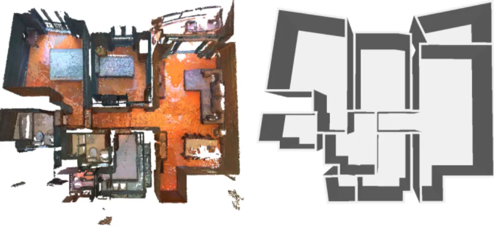
Figure 1: Goal of our approach. Left: the algorithm departs from raw point clouds as input data. Right: the floorplan of the indoor scene is reconstructed as a planar graph where each simple cycle represents the polygonal boundary of a room. Note that the 2D floorplan is converted into a 3D CAD model for visualization purpose.
at their exact positions,e.g., walls and corners [2]. Yet, industry still fully or
5
partially relies on human experts to generate high quality floorplans. Such in- teractive techniques, which requires an important manpower, cannot reasonably process large datasets of complex scenes.
We consider the task of reconstructing floorplan from point clouds by finding a planar graph where each simple cycle represents the polygonal boundary of
10
a room. Three main objectives are required in this task. First, geometric accuracy: we expect the geometric distance between the input points and the edges of planar graph as low as possible. In this way, recovering some small but important structure details of scenes is crucial for downstream applications, e.g.,indoor scene furnishing and reproduction. Second, topological guarantees:
15
the output planar graph must correspond to a series of connected, intersection- free polygons. Last,applicability: the proposed algorithm should be robust to various types of indoor scenes, in particular non-Manhattan scenes collected from different sensors,e.g., RGBD cameras and LIDAR scanners.
Reconstructing the floorplan from point clouds is usually operated in two
20
steps. First, somegeometric primitives are detected from input 3D data either
by traditional primitive detection methods [3, 4] or through learning approaches [5, 6]. These primitives locally describe the position of walls by planes or room corners by points, which form basic elements to represent the geometry of each room. Then, these primitives are assembled together to generate the associated
25
planar graph. A popular way is to directly connect these primitives through an optimization framework [7, 6]. This kind of methods are in general time- consuming and weakly robust in presence of under- and over-detection of primi- tives. Another strategy is to partition 2D space into polygonal facets and assign a room instance label to each facet [8, 9, 10]. This strategy is typically more
30
robust. However, it relies on an accurate estimation of room instance labeling map which might not be reachable in real applications.
We address these issues by designing a geometry processing method which relies on three main ingredients. First, we detect and regularize planes from the input data to locally capture parts of the walls. These planes are used to
35
generate a space partitioning data-structure that naturally provides a searching space in which the desired planar graph will be extracted. Second, we develop a constrained integer programming approach to capture the exact boundary shape with fine details. In this step, both the fidelity to input data and the complexity of the polygonal boundary are taken into account in a global energy
40
model. Such polygonal boundaries can be directly used in applicative scenarios, such as layout design [11, 12, 13]. Third, the inside area of the boundary shape is divided into different rooms by solving a multi-class labeling problem, which accounts for learned room instance label results and the positions of inside walls.
Figure 1 illustrates the goal of the proposed framework.
45
We demonstrate the potential of the algorithm on both RGBD and LIDAR scans, showing competitive results compared with (i) the current state-of-the- art floorplan generation methodFloorSP [6], (ii) the popular Douglas-Peucker algorithm [14], and (iii) a recent object vectorization approachASIP [10]
2. Related work
50
Our review of previous works covers four families of methods.
Vectorization pipelines. Reconstructing the floorplans from 3D points can be seen as extracting the contours of the room by chains of pixels in the point density image, and then simplifying them into polygons. Contours can be ex-
55
tracted for instance by popular object saliency detection methods [15, 16] or interactive techniques such as Grabcut [17]. The chains of these pixels form dense polygons that can be simplified to concise polygons by, for instance, the popular Douglas-Peucker algorithm [14] or edge contractions on Delaunay tri- angulation [18]. Unfortunately these vectorization pipelines cannot guarantee a
60
good topological accuracy as polygons are processed sequentially, without global consistency.
Partitioning-based methods. This strategy consists in detecting geometric primitives such as wall planes from point clouds and over-segmenting the 2D
65
space into polygonal facets. Then facets with the same room instance label are grouped together to form a polygonal room. Constrained Delaunay trian- gulation where the constrained edges are aligned with the walls can be used to detect interior triangles through line-of-sight information, before clustering the inside triangles into different rooms [19]. However, the presence of noisy
70
points on the wall components makes the output 3D model complex and not CAD-styled. Space partitioning data-structure is a popular tool to provide ba- sic geometric elements for recovering polygonal rooms. After dividing 2D space into polygonal facets, rooms are segmented either using an iterative clustering method [8], a global multi-class labeling approach [9] or an efficient greedy opti-
75
mization mechanism [10]. Note that all of these methods rely on room instance label of points to provide the semantic similarity between adjacent facets. This can be computed either through visibility information between points [20, 21]
or by a bottom-up approach [22]. These methods are influenced by noisy points
between adjacent rooms or individual objects inside each room, where points
80
located in the same room become invisible from each other due to unpredictable occlusions. In practice, these methods do not perform well on scenes with strong non-convexity.
Connectivity-based methods. Another intuitive solution is to connect the
85
detected isolated structure elements to form a planar graph. One popular ap- proach denoted as FloorNet [5] combines 2D features learned by DNN [23, 24]
and 3D features encoded by PointNet [25], inferring rich pixelwise geometric and semantic clues. These intermediate results are converted to a vector-graphic floorplan through a junction based integer programming framework [7]. This
90
pipeline achieves impressive results on large scale indoor scenes, but the set of predefined junction types cannot cover all room types in practice, in particular for non-Manhattan scenes. Also, the under-detection of corners easily lead to an erroneous topology in the floorplan graph. To address these issues, the current SOTA method known as FloorSP [6] employs Mask R-CNN [26] and DNN [23]
95
to provide room instance labeling results and corner/edge likelihood map. Then, a global energy combining these various information is formulated and solved by a room-wise coordinate descent algorithm. FloorSP brings a significant progress over previous methods, especially on strongly non-Manhattan scenes. Yet, note that this method relies on a post-processing step performed on image coordi-
100
nate, which is likely to lead to a miss-alignment between the final floorplan and the exact position of walls. Meanwhile, some structure details on the boundary shape cannot be fully captured with such a resolution-dependent representation.
Grammar based methods. Some works also address the floorplan recon-
105
struction task through grammar rules. One traditional solution is to build the structure graph of each element and then segment rooms with heuristics [2]. Connectivity information between rooms are also taken into account for segmenting rooms. The metrics, denoted as Potential Field distance [27], is computed for each voxel, before clustering the rooms in an hierarchical man-
110
ner. Another solution consists in reasoning on an adjacency graph of walls from which cycles of four connected walls are detected as a cuboid [28]. Rooms are then recovered by clustering cuboids according to their connection type. This method is however limited to Manhattan World scenes [29] in practice. More recently, data-driven approaches achieved successful results to recover 3D room
115
layout by processing the crucial information learned from the RGB Panorama such as floor-ceiling map and layout height map [30], boundary and corner map [31], as well as 1D layout representation [32]. These methods deliver clean re- sults for Manhattan-World scenes only.
120
Our approach is inspired by partitioning-based methods. However, in con- trast to [8], [9] and [10] which recover the floorplan graph only through a room- segmentation step, our method relies upon a more robust two-step mechanism that first extracts the boundary polygon of the scene and then divides the inside space into rooms.
125
3. Overview
Our algorithm takes as input a point cloud of real-world indoor scene and an associated pixelwise room instance labeling map [6], which is typically re- turned by state-of-the-art instance semantic segmentation techniques [26]. Our algorithm outputs a floorplan of the indoor scene under the form of a planar
130
graph where each simple cycle represents the polygonal boundary of a room.
The input point clouds are registered and the upward direction aligns the z- axis in world coordinate. We first convert the point cloud into a dense triangle mesh using standard method [33]. This conversion allows us to both operate on a lighter representation and be more robust to missing data and occlusions
135
massively found in point clouds describing indoor scenes.
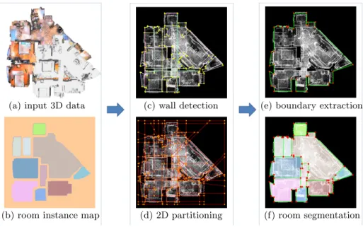
The algorithm operates in three steps as illustrated in Figure 2. First, a set of local geometric primitives,e.g., vertical planes, are detected by traditional shape detection methods [3, 4]. We filter and regularize the extracted planes to
(a) input 3D data
(b) room instance map
(c) wall detection
(d) 2D partitioning
(e) boundary extraction
(f) room segmentation
Figure 2: Overview of our approach. Our algorithm starts from a dense triangular mesh generated from the input point cloud (a) as well as an associated room instance labeling map (b). In the primitive detection step, a set of vertical planes that represent wall structures in the indoor scene are first extracted (c). After filtering and regularizing these wall planes, we partition the 2D X-Y space into a set of geometric elements,i.e.,vertices, edges and facets (d). Then the boundary edges of indoor scene are recovered by selecting a subset of edges (green ones) through solving a constrained integer programming formulation (e). Finally, the inside space of the indoor scene is divided into different areas (each colored polygonal facet), each of which represents a separated room (f). This step is performed by solving a multi-class labeling problem.
obtain a more regular plane configuration. Then, all the remaining wall planes
140
are projected onto the X-Y plane and used to partition the 2D space into a set of facets, edges and vertices (Section 4). Second, the boundary shape of indoor scene is recovered by choosing a subset of 2D-arrangement edges using a con- strained global energy minimization formulation (Section 5). This step enables us to divide the whole scene into inside and outside space. Finally, we assign a
145
label configuration to each facet inside the boundary by solving a Markov Ran- dom Field problem. Adjacent facets with the same label are grouped together and considered as a separated room (Section 6).
4. Primitive detection
150
As mentioned in Section 1, the most representative structures in the indoor scene are wall planes. They separate inside space from outside space, and divide adjacent rooms. So the first phase of our algorithm aims at extracting repre- sentative wall planes from a dense triangular mesh.
155
Plane extraction and filtering. We first detect all the planes using region growing method [3]. Each plane preserves the corresponding inlier triangular facets and vertices. Next, floor and ceiling planes are extracted among them, whose normal is quasi-parallel with z-axis and located close to the 3D bounding box. We reject the planespwhose normal vector is not quasi-orthogonal with
160
z-axis,i.e.,|−n→p· −→z|>0.1. The remaining planes are then considered as vertical planes. However, considering the often complex layout of indoor scenes, there may exist a few noisy planes that are not real parts of wall,e.g., vertical parts of furniture. To avoid the negative effect of these noisy vertical planes on the following operations, we filter out planes satisfying any of the following condi-
165
tions: (a) the number of inlier triangular facets is smaller than 2000; (b) the average distance between inlier vertices to plane is larger than 0.15m; (c) the minimum distance from inlier points to floor planes and ceiling planes is larger than 0.5m; (d) the area of inlier facets is smaller than 0.5m2. Up to now, all the remaining planes can be seen as wall components.
170
Plane regularization. Prior knowledge about the structure of the indoor scene should also be taken into consideration. In most cases, wall planes are straight-perpendicular to the floor and ceiling planes. So we reorient all the wall planes with a new normal straight-orthogonal to floor plane. We also fol-
175
low the hierarchical approach proposed in [34] to make the quasi-orthogonal (resp. quasi-parallel) plane pairs straight-orthogonal (resp. straight-parallel).
Finally, we merge coplanar wall planes if they are parallel or if the distance between them is smaller than 0.3m, as shown in Figure 2c.
180
2D space partition. Since the floorplan can be seen as a planar graph, where each room is a closed-loop, we discretize the 2D space into basic geometric ele- ments,i.e., vertices, edges and facets. To tackle this problem, we project wall planes onto the X-Y plane and partition the 2D space using a kinetic data- structure described in [35] (as illustrated in Figure 2d). As explained in [36],
185
this data structure allows to strongly reduce the solution space of the subse- quent steps compared to traditional arrangement techniques.
5. Boundary extraction
The objective of this step is to extract the boundary shape of the indoor
190
scene, which can best represent the contour of the indoor space. Note that the boundary shape should also conform to the manifoldness assumption, where each vertex is only connected to two adjacent edges. Given the set of edges E={ei|16i6n} generated in the previous step, we achieve this by selecting a subset of these edges using a constrained integer programming formulation.
195
We denote by xi ∈ {0,1}, a binary variable describing whether an edge ei∈ E is active (xi= 1) to be part of the boundary shape or not (xi= 0). The set of active edges composes the polygon boundary of the indoor scene. The quality of an activation state configurationx= (xi)i=1,2,...,nis measured by an energy of the form:
U(x) = (1−λ)Uf idelity(x) +λUcomplexity(x), (1) whereUf idelity(x) describes how well a state configurationxis consistent with the input data, while Ucomplexity(x) measures the complexity of the output boundary shape. Note that both terms are living in [0,1] and λ ∈ [0,1] is a parameter balancing these two terms.
200
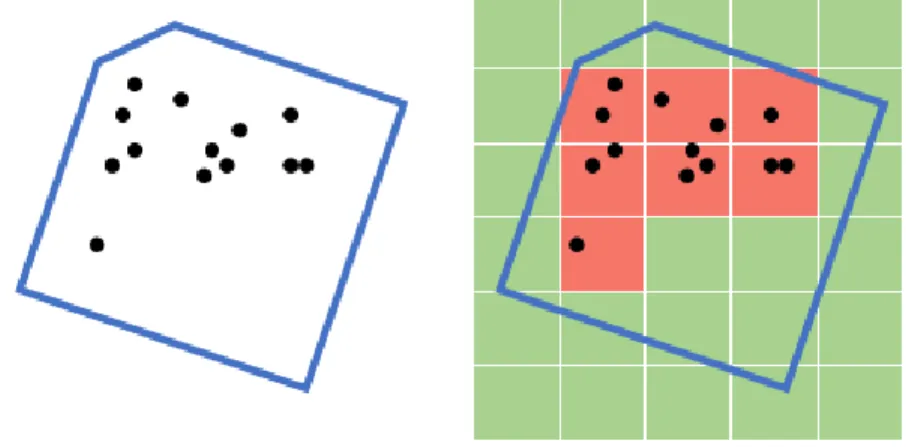
Figure 3: Probability of a facet to be labeled as inside. Left: we find all the points located inside a facet. Right: the 2D space is divided into an occupancy grid. The probability of a facet to be inside is given by the ratio of the number of the occupied cells to the number of cells inside the facet.
Fidelity term. Uf idelity(x) evaluates the coherence between active edges and the boundary shape. Because the boundary shape divides the whole space into inside and outside domains, we can observe that (i) most of the input points are located inside the boundary shape, and (ii) boundary edges highly overlap with wall structures. To fulfill these observations, our fidelity term is modeled as:
Uf idelity(x) =βUpoints(x) + (1−β)Uwalls(x). (2) The first termUpoints(x) measures the percentage of input points surrounded by the boundary edges, which is defined by:
Upoints(x) =
n
X
i=1
−|P(fi1)−P(fi2)| ·|ei|
Eˆ ·xi, (3) wherefi1, fi2 are two incident facets ofei and|ei| is the length ofei. ˆE is the total length of all the edges. P(.) measures the probability of one facet to be inside the boundary shape, as illustrated in Figure 3. Intuitively, Upoints(x) favors the selection of edges whose incident facets preserve different ratio of inside cells occupied by the input points. However, sinceUpoints(x) is negative, a lot of noisy edges will be active, even if the ratio difference is small. Thus,
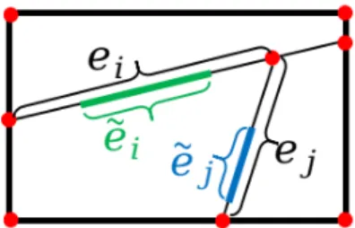
Figure 4: Overlapping segments|˜ei|,|˜ej|between each candidate edgeei,ej and the corre- sponding wall plane.
the second termUwalls(x) is designed to penalize such edges by measuring their overlapping part with the corresponding wall planes:
Uwalls(x) =
n
X
i=1
(1−|˜ei|
|ei|)·|ei|
Eˆ ·xi, (4)
where |˜ei| is the length of the segment of ei overlapping with corresponding wall plane as illustrated in Figure 4. Uwalls(x) assigns a large penalization for noisy edges that do not overlap with their associated wall planes. β ∈[0,1] is a parameter controlling the weight of these two terms. In our experiments, we set β = 0.5. In case of missing data or sparse distribution of input points, we
205
setβ= 0.7. In case of noise and outliers,β is set to 0.3.
Complexity term. In order to control the complexity of the final boundary shape, we introduce the complexity term defined as:
Ucomplexity(x) = 1
|V|
|V|
X
i=1
1{vi is corner}, (5) which has been used for surface reconstruction [37, 38]. V is the set of vertices computed in the previous step. The indicator returns true if (i) two incident edges of vertex vi are active, and (ii) these two edges originate from different
210
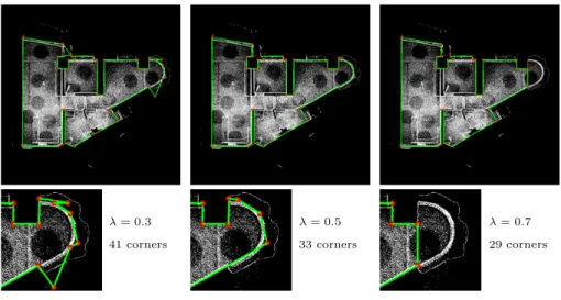
wall planes. This term favors returning a compact boundary shape polygon with a low number of corner vertices. Figure 5 illustrates how parameterλim- pacts the trade-off between data fidelity and output complexity. We typically fixλ= 0.5 in our experiments.
λ= 0.3 41 corners
λ= 0.5 33 corners
λ= 0.7 29 corners
Figure 5: Trade off between fidelity to data and complexity of the boundary shape. Whileλ increases, the output boundary shape contains less corner vertices.
215
Hard constraint. Because the output boundary shape should fulfill the man- ifoldness property, we must constrain each vertex of the boundary shape to contain two adjacent edges. We impose this with the following hard constraint:
X
ej∈Ev
xj = 0 or 2, ∀v∈V, (6)
whereEv is the set of edges adjacent to vertexv∈V.
Optimization. We search for the best activation state configuration x by minimizing the energy formulation in Eq.1 subjected to the constraint given in Eq.6. This constrained integer programming problem is solved by the SCIP
220
algorithm [39]. The active edges then compose the output boundary shape (see green edges in Figure 2e).
6. Room segmentation
The boundary shape recovered in previous step divides the 2D space into inside and outside domains. In this section, we only focus on the inside do- main and segment it into different rooms. Given the set of facets inside the boundary shape F = {fk|1 6 k 6 m}, we assign a room instance labeling L= (lk)k=1,2,...,mto each facet inF. In particular, we model this problem as a Markov Random Field approach via an energy of the standard form:
U(L) =
m
X
k=1
D(lk) +γ X
(j,k)∈E˜
V(lj, lk) (7)
whereD(lk) encodes unary term andV(lj, lk) encodes pairwise term. ˜Edenotes all pairs of adjacent inside facets.
225
Unary term. D(lk) is designed to encourage assigning each facet a label that is coherent with the input room instance labeling map:
D(lk) =−p
AklogP(lk), (8)
where Ak is the area of fk to measure the weight of each facet. P(lk) is the probability offk to be labeled aslk. P(lk) is computed as the ratio of number of pixels with valuelk in the input room instance labeling map to the number of pixels inside the facet.
230
Pairwise term. V(lj, lk) is designed for two purposes: (i) returning a low com- plexity floorplan, and (ii) separating rooms by wall planes inside the boundary shape. To do so, we penalize the edges whose adjacent facets preserve different room instance labels that do not overlap with its associated wall plane:
V(lj, lk) =
0 if lj=lk, (1−|˜|eei|
i|)· |ei| if lj6=lk,
(9)
whereei is the incident edge between facetsfj andfk. |˜ei| and|ei| retain the same definition as in Section 5. γis set to 1 to balance these two terms.
Room segmentation. Our proposed MRF model is solved by a standard
235
graph-cut optimization technique [40, 41]. We merge all the adjacent facets to one large polygon facet, each of which represents a room in the floorplan as shown in Figure 2f. Finally, we simplify the floorplan graph by removing vertices connected to two colinear edges. Note that there might be some skinny facets without any pixels with a non-background room instance label. In this case,
240
we optionally merge such facets to their adjacent rooms with longest common edge.
7. Experiments
Our algorithm has been implemented in C++, using the Computational Geometry Algorithms Library [42] to provide basic geometric tools. All the
245
experiments have been done on an Intel Core i7 CPU clocked at 3.6GHz.
Implementation details. Given the input point cloud, we compute the axis- aligned bounding box of all points projected onto the X-Y plane. We then extend the 2D bounding box by 0.5m and discretize it into a density map. Each
250
pixel value equals to 1 if there exists a point falling inside (see Figure 2c). Be- cause one of the most important goals of our approach is to recover a floorplan with detailed structures, we choose a fine resolution at 1cm. In this case, some small but important wall structures can also be recovered.
255
Evaluation metrics. We define the following metrics to evaluate and compare our results:
• Room metrics. As defined by Floorsp [6], a predicted room r is true- positive if and only if (i) r does not overlap with any other predicted room and (ii) there exists a ground truth room ˆr with IOU larger than
260
0.5 withr.
• Geometric metrics. Because most of the human-annotated ground truth floorplans do not exactly align with the real wall position (see column 3
of Figure 6), the geometric metrics between predicted models and ground truth cannot perfectly reflect the geometric accuracy of the proposed algo-
265
rithms. Thus, we convert 2D floorplans to a 3D CAD model and compute both the RMS and Chamfer distances between 3D model and input points.
Comparisons on RGBD scenes. We first compare our framework against the popular Douglas-Peucker algorithm [14], the object vectorization algorithm denoted as ASIP [10], and current state-of-the-art floorplan generation method
270
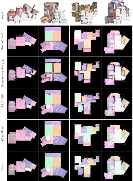
FloorSP [6] on 100 scenes collected from panorama RGBD scans. We employ the pre-trained model trained on 433 RGBD scenes released by FloorSP to provide the pixelwise room instance labeling map. Figure 6 illustrates the qualitative comparisons of various methods on hard cases, in particular on non Manhattan World scenes. ASIP and Douglas-Peucker output a set of isolated facets which is
275
caused by the disconnection of each region in the room instance labeling map.
In contrast, FloorSP is able to fill in this gap through a room-wise shortest path optimization strategy. Our method also returns a 2D planar graph by naturally recovering the boundary shape and dividing the inside domain into different polygonal facets. Also, since our method and ASIP capture the exact
280
position of walls in the scenes, the reconstructed floorplans align better with input data than FloorSP and Douglas-Peucker. Finally, our floorplan maintains more structure details than the other methods thanks to our boundary shape extraction mechanism.
Quantitatively, Figure 7 illustrates the geometric accuracy of each method.
285
Our algorithm gives the lowest Chamfer distance between input points and output models thanks to the preservation of small details. Moreover, Table 1 spotlights the average evaluation metrics and Figure 8 shows the distribution of geometric metrics of all methods on 100 RGBD scenes. Our method delivers the best score on room metrics. This progress mainly comes from our two-step
290
reconstruction approach which combines the distribution of points, the positions of wall planes and the room instance labeling map together. In contrast, the other methods are less robust to defects contained in room instance labeling
InputGroundtruthDouglas-Peucker[14]ASIP[10]FloorSP[6]Ours
Figure 6: Qualitative comparisons on RGBD scenes. Douglas-Peucker and ASIP return a set of isolated facets while FloorSP and our method produce a valid connected graph. In term of geometric accuracy, floorplans of ASIP and our approach align better with input points than FloorSP and Douglas-Peucker, especially in case of non-Manhattan scenes. In particular, our method achieves to preserve small structure details.
0
≥0.5m InputDouglas-Peucker[14]ASIP[10]FloorSP[6]Ours
e: 0.079 t: 0.3s
e: 0.082 t: 1.5s
e: 0.096 t: 188s
e: 0.074 t: 13s
e: 0.163 t: 0.2s
e: 0.144 t: 1.8s
e: 0.194 t: 228s
e: 0.143 t: 10s
e: 0.156 t: 0.2s
e: 0.125 t: 1.9s
e: 0.190 t: 289s
e: 0.122 t: 11s
Figure 7: Comparisons on RGBD scenes. We convert the output 2D floorplan of each method into a 3D CAD model with wall thickness equals to 0.1m. The red-to-blue colored points encode the Chamfer distance between the corresponding input points and the 3D CAD models.
Douglas-Peucker and ASIP give a relatively lower error within a few seconds while returning a set of non-connected rooms. FloorSP outputs a simple floorplan and 3D CAD model, yet, some wall structures are a bit far away from the input data (see blue points on the vertical walls). By preserving some fine details, our method returns the best error. Moreover, our method is faster than FloorSP by approximately one order of magnitude.
Figure 8: Histogram of geometric metrics on 100 RGBD scenes. While most of the scenes are located in the first two bins for the four methods, our method is the most accurate: FloorSP has a lower number of scenes contained in the first bin while Douglas-Peucker and ASIP produce models with relatively large geometric errors on the last bins.
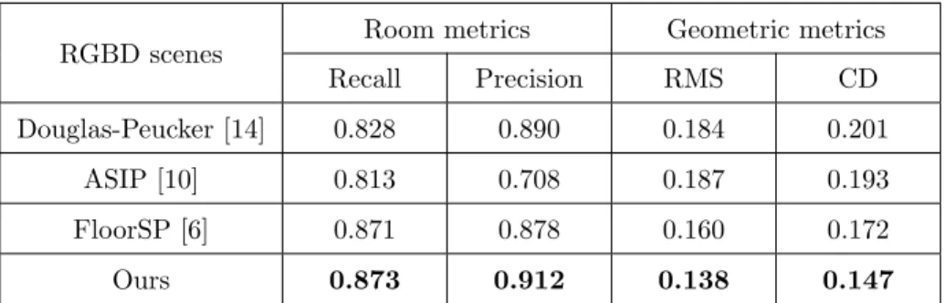
RGBD scenes
Room metrics Geometric metrics
Recall Precision RMS CD
Douglas-Peucker [14] 0.828 0.890 0.184 0.201
ASIP [10] 0.813 0.708 0.187 0.193
FloorSP [6] 0.871 0.878 0.160 0.172
Ours 0.873 0.912 0.138 0.147
Table 1: Quantitative comparison on 100 RGBD scenes. RMS and CD refer to the RMS distance and the Chamfer distance, expressed in meter.
maps. Besides, for geometric metrics, our method also achieves the minimum RMS and Chamfer errors. These scores can be explained by the robustness of
295
our two-step optimization strategy which encourages the floorplan to align well even with the small wall components. We also provide a supplementary material to show more qualitative and quantitative comparisons.
Comparisons on LIDAR scenes. To evaluate the robustness of each method
300
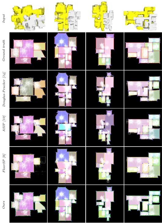
on different source of sensors, we also collect 88 production-level indoor scenes scanned by LIDAR. Qualitatively, Figure 9 shows the floorplans reconstructed
InputGroundtruthDouglas-Peucker[14]ASIP[10]FloorSP[6]Ours
Figure 9: Qualitative comparisons on LIDAR scenes. Our algorithm is less influenced by wrong room instance labeling map caused by different source of scans than the other methods.
0
≥0.5m InputDouglas-Peucker[14]ASIP[10]FloorSP[6]Ours
e: 0.128 t: 0.2s
e: 0.127 t: 2.0s
e: 0.149 t: 394s
e: 0.120 t: 13s
e: 0.101 t: 0.2s
e: 0.097 t: 1.5s
e: 0.110 t: 157s
e: 0.087 t: 11s
e: 0.160 t: 0.3s
e: 0.169 t: 5.3s
e: 0.179 t: 264s
e: 0.129 t: 14s
Figure 10: Comparisons on LIDAR scenes. Douglas-Peucker and ASIP are quite efficient for generating a set of non-connected polygons. Although FloorSP outputs simple planar graphs with correct topology, its geometric error and the computational time is relatively high. Our method generates 3D models that best align with the wall points (see the distribution of colored points on vertical structures).
Figure 11: Histogram of geometric metrics on 88 LIDAR scenes. Similarly to results obtained from RGBD data, our algorithm produces more accurate models from Lidar scans than ASIP, FloorSP and Douglas-Peucker methods. In particular, the errors of our models mostly range in the two first bins of the histograms.
LIDAR scenes
Room metrics Geometric metrics
Recall Precision RMS CD
Douglas-Peucker [14] 0.621 0.840 0.250 0.251
ASIP [10] 0.698 0.746 0.173 0.169
FloorSP [6] 0.703 0.865 0.189 0.187
Ours 0.714 0.872 0.137 0.136
Table 2: Quantitative comparison on 88 LIDAR scenes.
from LIDAR points by each method. We can draw similar conclusions about the quality of output floorplans returned by all methods as shown in Figure 6. Our algorithm still outperforms the other methods in terms of geometric accuracy.
305
Quantitatively, Figure 10 illustrates the geometric metrics between 3D mod- els generated by each method and input points. Our algorithm outperforms the other methods since our 3D planar graph is reconstructed from detected walls where some small but significant structure details in the scene are successfully recovered. Table 2 and Figure 11 provide the average metric scores and their
310
distribution for the four methods from the LIDAR dataset respectively. As for RGBD data, our method achieves the best evaluation scores. Additional com-
room label map ours one-step ours two-step
Figure 12: Ablation study. Directly performing room segmentation on room instance label map misses recovering some rooms (top) or generates an isolated graph (bottom). In contrast, our two-step approach does not suffer from this problem by first reconstructing the boundary shape from input point distribution (which is not related to inexact room instance label map).
parison results are illustrated in supplementary material.
Ablation study. In contrast to previous room segmentation methods based
315
on one-step optimization approach [8, 9, 10], one of the most significant ingre- dients of our system lies in reconstructing the floorplan in a two-step manner:
boundary extraction then room segmentation. We study the robustness of our two-step approach against the one-step approach which skips the boundary ex- traction process in Figure 12. Two types of errors occur when using a one-
320
step method: (i) several rooms are incorrectly labeled as background, and (ii) some rooms are isolated where polygonal facets between them are labeled as background. Our two-step mechanism is less affected by these errors by first recovering the boundary shape which does not rely on room instance label. We
Col 1 of Figure 6
Col 4 of Figure 6
Col 1 of Figure 9
Col 3 of Figure 9
# points of input point cloud 481K 1280K 973K 1498K
# facets of raw mesh 230K 283K 343K 221K
# wall planes 35 53 39 31
# candidate edges inE 266 402 380 316
# selected boundary edges 55 53 82 51
# inside facets in F 32 63 22 48
# polygonal rooms 4 8 6 9
Primitive detection time (s) 6.7 8.4 10.2 7.1
Boundary extraction time (s) 1.0 1.7 1.5 1.3
Room segmentation time (s) 0.9 1.1 0.4 0.8
Memory peak (MB) 197 393 339 503
Table 3: Performance of our algorithm on various RGBD and LIDAR data.
compared these two strategies on 30 scenes. For one-step method, we retrieve
325
a score of 0.64 and 0.69 on room recall and precision with IOU=0.7 to ground truth. However, for our two-step method, we obtain a higher score of 0.71 and 0.74 on these two metrics.
Performances. Table 3 shows the performances of our algorithm in terms of
330
processing time and memory consumption on several indoor scenes. Primitive detection is the most time-consuming step, typically around 70% of the total running time. The subsequent boundary extraction and room segmentation steps are much faster. Indeed, these steps rely on an integer programming approach and a graph-cut formulation in which only a few hundreds of candidate
335
edges and dozens of insides facets are involved respectively. This efficiency originates from the high compactness of the kinetic data-structure.
Evaluation on the ISPRS benchmark. We also evaluate our method on the
0
≥0.5m
CaseStudy1CaseStudy5
input data our result
e: 0.010 t: 10s F: 68K
e: 0.023 t: 14s F: 159K
Figure 13: Results on the ISPRS benchmark. The reconstructed models are accurate and allow rooms and corridors to be described with an highly-compact piecewise-planar representation.
CaseStudy 1 and CaseStudy 5 of ISPRS benchmark on indoor modeling [43].
340
For performance reasons, we down-sample the original point clouds to 2.4M and 2.9M points forCaseStudy 1 andCaseStudy 5 respectively. As illustrated in Figure 13, since the room instance labeling map is obtained by employing the Mask R-CNN model which is pre-trained on RGBD scenes, some adjacent rooms are segmented to one. However, our boundary extraction step succeeds
345
in recovering the correct boundary shape of two scenes while preserving small vertical structures, which demonstrates the applicability of our method on var- ious sources of data.
Robustness to furniture and cluttered elements. In our experiments, the
350
collected indoor scenes typically contain furniture such as chairs, desks or plants.
As illustrated in Figure 14, our algorithm allows us to filter out such elements for two reasons. First, our primitive detection step filters out some non-wall planes according to prior knowledge on indoor scenes. This step ensures that most of the furniture will be ignored for the subsequent steps. Second, when
355
vertical parts of furniture are wrongly detected as wall planes, the subsequent boundary extraction and room segmentation steps exploit various types of in-
input data 42 detected wall planes our result
Figure 14: Influence of furniture. Despite the erroneous detection of planes on furniture components, our algorithm remains robust to recover the boundary shape of indoor scene and decompose the inside space into separated rooms (see the red marked regions in the middle sub-figure).
formation such as the distribution of points, the position of walls or the room instance labeling map that contribute to reduce the effect of planes detected on furniture.
360
Limitations. Our system relies on two crucial clues: (i) the room instance label map returned by Mask R-CNN, and (ii) the detected wall planes. As illustrated in Figure 15, these two ingredients, when imprecise, can lead to output models with geometric errors. Room instance label map plays an important role for
365
room segmentation. Although our formulation is quite robust while handling some miss-labeling on the boundary of each room, a large miss-labeled region can lead to a bad room segmentation result, even if the boundary shape of scene is correctly reconstructed. Also, the boundary shape shrinks when some large walls are missed because of either false-negative in the plane detection or
370
false-positive in the plane filtering.
8. Conclusion
We proposed an automatic algorithm to reconstruct floorplan from point clouds of indoor scenes. Our method starts by detecting wall planes to parti-
Failurecase2Failurecase1
wall planes room label map
our result our result
ground truth ground truth
Figure 15: Failure cases. Two sources of typical failure cases contained in our framework: (i) wrong input room label map (top), and (ii) missing wall planes (bottom).
tion the space into geometric elements. Then the boundary shape is recovered
375
through a constrained integer programming formulation. The inside domain is then segmented into rooms by solving a multi-class labeling mechanism. We demonstrated the flexibility and robustness of our method on both RGBD and LIDAR scans from simple to complex cases, and its competitiveness with respect to the state-of-the-art methods.
380
There are several aspects to improve in future work. First, the splitting operator proposed in ASIP [10] can be applied to potentially solve the issue of missing wall planes. Second, we would like to exploit the normal vector of points and visibility information to reduce the impact of imprecise input room instance label map. Finally, we could also generalize our method to extract the
385
shape of free-form scenes through detecting higher-order geometric primitives.
9. Acknowledgments
This work was supported in parts by NSFC (U2001206), DEGP Key Project
(2018KZDXM058), Shenzhen Science and Technology Program (RCJC20200714114435012) and Beike (https://www.ke.com). The authors are grateful for the data and an-
390
notation tools from Beike, and also thank Muxingzi Li for technical discussions.
[1] G. Pintore, C. Mura, F. Ganovelli, L. J. Fuentes-Perez, R. Pajarola, E. Gob- betti, State-of-the-art in Automatic 3D Reconstruction of Structured In- door Environments, Computer Graphics Forum.
[2] S. Ikehata, H. Yang, Y. Furukawa, Structured indoor modeling, in: Proc.
395
of International Conference on Computer Vision (ICCV), 2015.
[3] T. Rabbani, F. van Den Heuvel, G. Vosselman, Segmentation of point clouds using smoothness constraint, ISPRS 36.
[4] R. Schnabel, R. Wahl, R. Klein, Efficient ransac for point-cloud shape detection, Computer Graphics Forum 26.
400
[5] C. Liu, J. Wu, Y. Furukawa, Floornet: A unified framework for floorplan reconstruction from 3d scans, in: Proc. of European Conference on Com- puter Vision (ECCV), 2018.
[6] J. Chen, C. Liu, J. Wu, Y. Furukawa, Floor-sp: Inverse cad for floorplans by sequential room-wise shortest path, in: Proc. of International Conference
405
on Computer Vision (ICCV), 2019.
[7] C. Liu, J. Wu, P. Kohli, Y. Furukawa, Raster-to-vector: Revisiting floor- plan transformation, in: Proc. of International Conference on Computer Vision (ICCV), 2017.
[8] C. Mura, O. Mattausch, A. J. Villanueva, E. Gobbetti, R. Pajarola, Auto-
410
matic room detection and reconstruction in cluttered indoor environments with complex room layouts, Computers & Graphics 44 (2014) 20–32.
[9] S. Ochmann, R. Vock, R. Wessel, R. Klein, Automatic reconstruction of parametric building models from indoor point clouds, Computers & Graph- ics 54 (2016) 94–103.
415
[10] M. Li, F. Lafarge, R. Marlet, Approximating shapes in images with low- complexity polygons, in: Proc. of Computer Vision and Pattern Recogni- tion (CVPR), 2020.
[11] W. Wu, L. Fan, L. Liu, P. Wonka, Miqp-based layout design for building interiors, Computer Graphics Forum 37 (2018) 511–521.
420
[12] W. Wu, X. Fu, R. Tang, Y. Wang, Y. Qi, L. Liu, Data-driven interior plan generation for residential buildings, ACM Transactions on Graphics.
[13] R. Hu, Z. Huang, Y. Tang, O. Van Kaick, H. Zhang, H. Huang, Graph2plan:
Learning floorplan generation from layout graphs, ACM Transactions on Graphics 39.
425
[14] S. T. Wu, M. R. G. Marquez, A non-self-intersection douglas-peucker algo- rithm, in: IEEE Symposium on Computer Graphics and Image Processing, 2003.
[15] M.-M. Cheng, N. J. Mitra, X. Huang, P. H. S. Torr, S.-M. Hu, Global con- trast based salient region detection, IEEE Transactions on Pattern Analysis
430
and Machine Intelligence 37 (2015) 569–582.
[16] G. Li, Y. Yu, Deep contrast learning for salient object detection, in: Proc.
of Computer Vision and Pattern Recognition (CVPR), 2016.
[17] C. Rother, V. Kolmogorov, A. Blake, Grabcut: Interactive foreground ex- traction using iterated graph cut, ACM Transactions on Graphics 23.
435
[18] C. Dyken, M. Dæhlen, T. Sevaldrud, Simultaneous curve simplification, Journal of Geographical Systems 11 (2009) 273–289.
[19] E. Turner, A. Zakhor, Floor plan generation and room labeling of indoor environments from laser range data, in: Proc. of International Conference on Computer Graphics Theory & Applications (GRAPP), 2015.
440
[20] S. Ochmann, R. Vock, R. Wessel, M. Tamke, R. Klein, Automatic gen- eration of structural building descriptions from 3d point cloud scans, in:
Proc. of International Conference on Computer Graphics Theory and Ap- plications (GRAPP), 2014.
[21] R. Ambrus, S. Claici, A. Wendt, Automatic room segmentation from un-
445
structured 3d data of indoor environments, IEEE Robotics and Automation Letters 2 (2017) 749–756.
[22] I. Armeni, O. Sener, A. Zamir, H. Jiang, I. Brilakis, M. Fischer, S. Savarese, in: Proc. of Computer Vision and Pattern Recognition (CVPR), 2016.
[23] F. Yu, V. Koltun, T. Funkhouser, Dilated residual networks, in: Proc. of
450
Computer Vision and Pattern Recognition (CVPR), 2017.
[24] A. Newell, K. Yang, J. Deng, Stacked hourglass networks for human pose estimation, arXiv preprint arXiv:1603.06937.
[25] R. Q. Charles, H. Su, M. Kaichun, L. J. Guibas, Pointnet: Deep learning on point sets for 3d classification and segmentation, in: Proc. of Computer
455
Vision and Pattern Recognition (CVPR), 2017.
[26] K. He, G. Gkioxari, P. Doll´ar, R. Girshick, Mask r-cnn, in: Proc. of Inter- national Conference on Computer Vision (ICCV), 2017.
[27] D. Bobkov, M. Kiechle, S. Hilsenbeck, E. Steinbach, Room segmentation in 3d point clouds using anisotropic potential fields, in: Proc. of International
460
Conference on Multimedia and Expo, 2017.
[28] S. Murali, P. Speciale, M. R. Oswald, M. Pollefeys, Indoor scan2bim: Build- ing information models of house interiors, in: Proc. of Intelligent Robots and Systems (IROS), 2017.
[29] Y. Furukawa, B. Curless, S. M. Seitz, R. Szeliski, Manhattan-world stereo,
465
in: Proc. of Computer Vision and Pattern Recognition (CVPR), 2009.
[30] S.-T. Yang, F.-E. Wang, C.-H. Peng, P. Wonka, M. Sun, H.-K. Chu, Dula- net: A dual-projection network for estimating room layouts from a sin- gle rgb panorama, in: Proc. of Computer Vision and Pattern Recognition (CVPR), 2019.
470
[31] C. Zou, A. Colburn, Q. Shan, D. Hoiem, Layoutnet: Reconstructing the 3d room layout from a single rgb image, in: Proc. of Computer Vision and Pattern Recognition (CVPR), 2018.
[32] C. Sun, C.-W. Hsiao, M. Sun, H.-T. Chen, Horizonnet: Learning room layout with 1d representation and pano stretch data augmentation, in:
475
Proc. of Computer Vision and Pattern Recognition (CVPR), 2019.
[33] M. Kazhdan, H. Hoppe, Screened poisson surface reconstruction, ACM Transactions on Graphics 32 (2013) 1–13.
[34] Y. Verdie, F. Lafarge, P. Alliez, LOD Generation for Urban Scenes, ACM Transactions on Graphics 34.
480
[35] J.-P. Bauchet, F. Lafarge, KIPPI: KInetic Polygonal Partitioning of Images, in: Proc. of Computer Vision and Pattern Recognition (CVPR), 2018.
[36] J.-P. Bauchet, F. Lafarge, Kinetic Shape Reconstruction, ACM Trans. on Graphics 39 (5).
[37] L. Nan, P. Wonka, Polyfit: Polygonal surface reconstruction from point
485
clouds, in: Proc. of International Conference on Computer Vision (ICCV), 2017.
[38] H. Fang, F. Lafarge, Connect-and-Slice: an hybrid approach for recon- structing 3D objects, in: Proc. of Computer Vision and Pattern Recogni- tion (CVPR), 2020.
490
[39] P. Fouilhoux, A. Questel, Scip: solving constraint integer programs, RAIRO - Operations Research 48 (2014) 167–188.
[40] Y. Boykov, O. Veksler, R. Zabih, Fast approximate energy minimization via graph cuts, IEEE Transactions on Pattern Analysis and Machine Intel- ligence 23 (2002) 1222–1239.
495
[41] Y. Boykov, V. Kolmogorov, An experimental comparison of min-cut/max- flow algorithms for energy minimization in vision, IEEE Transactions on Pattern Analysis and Machine Intelligence 26 (9) (2004) 1124–1137.
[42] Cgal, Computational Geometry Algorithms Library, http://www.cgal.org.
[43] K. Khoshelham, L. D. Vilari˜no, M. Peter, Z. Kang, D. Acharya, The isprs
500
benchmark on indoor modelling, Int. Arch. Photogramm. Remote Sens.
Spat. Inf. Sci 42 (2017) 367–372.