[PENDING] Gratings: Theory and Numeric Applications

(1)

Gratings:

Theory and Numeric Applications

Second Revisited Edition

Tryfon Antonakakis Fadi Baïda

Abderrahmane Belkhir Kirill Cherednichenko Shane Cooper

Richard Craster Guillaume Demesy John DeSanto

Gérard Granet

Evgeny Popov, Editor

Boris Gralak Leonid Goray

Sébastien Guenneau Lifeng Li

Daniel Maystre André Nicolet Gunther Schmidt Brian Stout

Fréderic Zolla

Institut Fresnel, Université d’Aix-Marseille, Marseille, France

Institut FEMTO-ST, Université de Franche-Comté, Besançon, France Institut Pascal, Université Blaise Pascal, Clermont-Ferrand, France Colorado School of Mines, Golden, USA

CERN, Geneva, Switzerland Imperial College London, UK Cardiff University, Cardiff, UK

Université Mouloud Mammeri, Tizi-Ouzou, Algeria

Saint Petersburg Academic University, Saint Petersburg, Russian Federation Institute for Analytical Instrumentation, Saint Petersburg, Russian Federation Weierstrass Institute of Applied Analysis and Stochastics, Berlin, Germany Tsinghua University, Beijing, China

ISBN: 978-2-85399-943-4

www.fresnel.fr/numerical-grating-book-2

(2)

ISBN: 2-85399-943-4

Second Edition, 2014

World Wide Web:

www.fresnel.fr/numerical-grating-book-2

Aix Marseille Université, CNRS, Centrale Marseille, Institut Fresnel UMR 7249, 13397 Marseille,

France

Gratings: Theory and Numeric Applications, Second Revisited Edition, Evgeny Popov, editor (Aix Marseille Université, CNRS, Centrale Marseille, Institut Fresnel UMR 7249, 2014)

2014

Presses Universitaires de Provence

(3)

Chapter 12:

Boundary Integral Equation Methods for Conical Diffraction and Short Waves

Leonid I. Goray and Gunther Schmidt

(4)

12.1 Introduction . . . 1

12.2 Integral method for one-profile gratings in conical diffraction . . . 2

12.2.1 Maxwell equations . . . 3

12.2.2 Helmholtz equations . . . 4

12.2.3 Boundary integral operators . . . 7

12.2.4 Integral equations for the in-plane case . . . 10

12.2.5 Formulas for Rayleigh coefficients . . . 12

12.2.6 Integral equations for the off-plane case . . . 13

12.3 Efficiency, absorption, and energy balance . . . 15

12.3.1 Efficiencies in conical diffraction . . . 15

12.3.2 Generalization of energy balance for absorbing bare gratings . . . 18

12.3.3 Absorption for bare gratings . . . 19

12.3.4 Efficiencies and absorption for in-plane diffraction . . . 20

12.4 Numerical solution of single-boundary problems . . . 20

12.4.1 Mathematical results for the integral equations . . . 20

12.4.2 Approximation of integral equations . . . 21

12.4.3 Nyström discretization with modifications . . . 24

12.4.4 Hybrid trigonometric-spline collocation . . . 25

12.4.5 Evaluations of kernels . . . 27

12.4.6 Cache for exponential functions (plane waves) . . . 31

12.5 Solving diffraction of multilayer gratings . . . 32

12.5.1 Gratings with separating boundaries . . . 33

12.5.2 Determination of the scattering matrices . . . 35

12.5.3 Gratings with penetrating boundaries . . . 37

12.5.4 Generalization of energy balance for lossy multilayer gratings . . . 40

12.6 Implementation and algorithmic enhancements of multilayer solvers . . . 41

12.6.1 Implementation of multilayer schemes . . . 42

12.6.2 Cache for kernel functions . . . 43

12.6.3 Cache for repeating pairs or quads of layers . . . 44

12.7 Modifications of integral methods for very small wavelength-to-period ratios . . 45

12.7.1 Approximations . . . 46

12.7.2 Convergence and accuracy with and without speed-up technique . . . . 47

12.7.3 Summation rules for kernel functions and energy balance . . . 53

12.8 Analysis of rough gratings using quasi-periodicity and Monte Carlo calculus . . 55

12.8.1 Scattering intensity, absorption, and energy balance of rough 1D gratings 56 12.8.2 Scattering intensity of rough gratings in a dispersive plane . . . 58

12.8.3 Scattering intensity of rough gratings in a non-dispersive plane . . . 59

12.9 Examples of numerical results . . . 60

12.9.1 Efficiencies and polarization angles of lamellar gratings . . . 62 1

(5)

12.9.4 Anomalously absorbing Ag shallow-sine grating in the visible . . . 63 12.9.5 Photonic crystals with Au nanorods in the visible–near-IR . . . 64 12.9.6 Lossless photonic crystal with circular rods in the near- and mid-IR . . 66 12.9.7 Al echelle grating coated by MgF₂in the VUV . . . 68 12.9.8 Au off-plane-grazing-incidence blaze grating in soft x-rays . . . 70 12.9.9 W/B₄C multilayer off-plane-grazing-incidence blaze grating in soft-x-

rays . . . 71 12.9.10 Flight Mo/Si multilayer rough lamellar grating in the EUV . . . 73 12.10Appendix A: Derivation of the recursive algorithm for Separating solver . . . . 75 12.11Appendix B: Derivation of the recursive algorithm for Penetrating solver . . . . 77 12.12Appendix C: Derivation of the absorption energy for multilayer gratings . . . . 79 12.13Appendix D: Derivation of the general connection rule between 2D and 1D

gratings . . . 81

(6)

(7)

Boundary Integral Equation Methods for Conical Diffraction and Short Waves

Leonid I. Goray

^(1,2)

and Gunther Schmidt

⁽³⁾

(1)Saint Petersburg Academic University, RAS, Khlopin 8/3, St. Petersburg 194021, Russian Federation, goray@spbau.ru,

(2)Institute for Analytical Instrumentation, RAS, Ivana Chernykh 31-33, St. Petersburg 198095, Russian Federation,lig@pcgrate.com,

(3)Weierstrass Institute of Applied Analysis and Stochastics, Mohrenstrasse 39, Berlin 10117, Germany, schmidt@wias-berlin.de

12.1 Introduction

This work is part of research that has been pursued by the authors over a long period of time for the purpose of developing accurate and fast numerical algorithms, including the commercial packages PCGrate and DiPoG [12.1, 12.2] designed to model multilayered gratings having mostly one-dimensional periodicity (1D), including roughness, and working in all, including the shortest, optical wavelength ranges at arbitrary optical mounts.

The boundary integral equation theory or, briefly, integral method (IM) is presently uni- versally recognized as one of the most developed and flexible approaches to an accurate numerical solution of diffraction grating problems (see, e.g., Ref. 12.3 and Ch. 4 and references therein). Viewed in the historical context, this method was the first to offer a solution to vector problems of light diffraction by optical gratings and to demonstrate remarkable agreement with experimental data. This should be attributed to the high accuracy and good convergence of the method, especially for the TM polarization plane. It does not involve limitations similar to those characteristic of the Coupled-Wave Analysis (CWA), and it provides a better convergence. The disadvantages of this method include its being mathematically complicated, as well as numerous "peculiarities" involved in numerical realization. In particular, quasi-periodic Greens functions and their derivatives appearing as kernels in the integral operators require sophisticated lattice sum techniques to evaluate. Moreover, application of the IM to cases of heterogeneous or anisotropic media meets with difficulties; however, with the volume integral method it is possible to overcome these difficulties easily. Nevertheless, it is on the basis of this theory that all the well-known problems of diffraction by periodic and non-periodic structures in optics and other fields have been solved. In many cases it offers the only possible way to follow up in research. The flexibility and universality inherent in the IM, in particular, enable

(8)

one rather easily to reduce the problem of radiation of Gaussian waves or of a localized source to that of plane-wave incidence, for which scientists all over the world have a set of numerical solutions. Generalizations of the IM have recently been proposed for arbitrarily profiled 1D multilayer gratings [12.4], randomly-rough x-ray-extreme-ultraviolet (EUV) gratings and mir- rors [12.5, 12.6], conical diffraction gratings including materials with a negative permittivity and permeability (metamaterials) [12.7, 12.8], bi-periodic anisotropic structures using a vari- ation formulation [12.9], Fresnel zone plates and diffraction optical elements [12.10, 12.11], and two-dimensional (2D) [12.12, 12.13] and three-dimensional (3D) [12.14] photonic crystals (inclusions) of some geometries, among others.

The IM is so pivotal that one can indicate the few areas where it can be modified and im- proved to solve particular diffraction problems. By convention they are: (1) physical model—

choice of boundary types, boundary conditions, layer and substrate refractive indices, and radiation conditions; (2) mathematical structure—integral representations using potentials or integral formulas and a multilayer scheme; (3) method of approximation and discretization—

discretization schemes, choice of basis (trial) and test (weighting) functions, and treatment of coincident points and corners in boundary profile curves; (4) low-level details—calculations and optimization of kernel functions, mesh of discretization (collocation) points, quadrature rules, and solution of linear algebraic systems; (5) implementation enhancements—memory caching, other implementation details. A self-consistent explanation of the existing IMs is beyond the primary scope of the present study. The main purpose of this Chapter is to present a complete description in general operator form of the two IMs applied to 1D multilayer gratings working in conical diffraction mounts and in short waves. Our study also includes the calculus of grating absorption in the explicit form and scattering intensity of randomly-rough gratings using Monte Carlo simulations. For other formal IM treatments and their comparisons, one should rather look to the references of this Chapter as well as to Ch. 4 and to references therein.

Various kinds of electromagnetic features of different nature can exist and be explored in complex grating structures: Bragg and Brewster resonances, Rayleigh anomalies and groove shape features, waveguiding and Fano-type modes, etc. In conical diffraction, the influence of possible types of waves can be mixed. For the purposes of this Chapter, we chose three important types, among many others, of diffraction grating problems to include them in Section 12.9

"Examples of numerical results". They are: bare dielectric or metallic gratings of standard groove shapes working in conical diffraction in the resonance domain; shallow high-conductive or dielectric gratings of various boundary shapes, including closed ones, working in different mounts and supporting polariton-plasmon excitation or Bragg diffraction in the visible–infrared range; bare and multilayer gratings working in grazing-conical or near-normal in-plane diffraction in the soft x-ray–EUV range.

12.2 Integral method for one-profile gratings in conical diffraction

The present IM designed for the calculation of the efficiency of bulk and multilayer gratings with arbitrary boundary shapes including micro- and nanoroughness and over an extremely wide wavelength range is considered here in a general operator formalism. In this Section, we consider single-boundary integral equations, which involve boundary integrals of the single and double layer potentials and also the normal and tangential derivatives of single layer potentials.

Analytical aspects of boundary integral operators are well represented in publications and, the most relevant of them for the present study, are also in following Sections. The fields are assumed time harmonic. Under these conditions, in classical (in-plane) diffraction the Maxwell

(9)

system of equations reduces to a single Helmholtz equation; therefore fields are represented in the sequel by scalar functions. They would be vector functions with two components in the case of conical (off-plane) diffraction. In the present Section, we are concerned mostly with conical diffraction, including some notes about metamaterials. Classical diffraction is considered as a particular case with some important details for the implementation.

There exist different ways to transform the diffraction problems under consideration to one-dimensional integral equations over the boundary profile curve of the grating. It is beyond the scope of this chapter to describe the history of applying integral methods to grating problems and the variety of corresponding integral formulations. It should be mentioned that those methods were mostly developed by specialists in physics and optics, and, it seems, they were not aware of the rapid progress in the fields of "boundary integral equations" and "boundary element methods" made in the mathematical community since 1980.

12.2.1 Maxwell equations

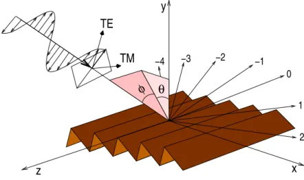
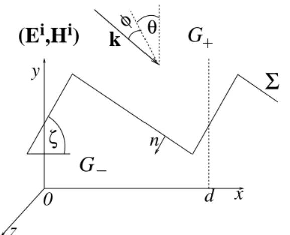
We denote bye_x,e_yande_zthe unit vectors of the axis of the Cartesian coordinates. The grating is a cylindrical surface whose generatrices are parallel to thez-axis (see Fig. 12.1) and whose cross section is described by the curveΣ(Fig. 12.2). We suppose thatΣis not self-intersecting andd- periodic inx-direction. The grating surface is the boundary between two regionsG_±×R⊂R³ which are filled with materials of constant electric permittivity ε± and magnetic permeability µ±. We deal only with time-harmonic fields; consequently, the electric and magnetic fields are

x y

2 1

−4 −3 −1

0

−2

TE

z

TM θ φ

Figure 12.1: Schematic conical diffraction by a grating.

represented by the complex vectorsEandH, with a time dependence exp(−iω^t)taken into ac- count. The wave vectork+of the incident wave inG+×Ris in general not perpendicular to the grooves (k₊·ez̸=0). Settingk+= (α^,−β^,γ⁾the surface is illuminated by an electromagnetic plane wave

Eⁱ=peⁱ⁽^α^x^−β^y+^γ^z), Hⁱ=seⁱ⁽^α^x^−β^y+^γ^z), (12.1) which due to the periodicity of Σis scattered into a finite number of plane waves in G₊×R and possibly inG₋×R. The wave vectors of these outgoing modes lie on the surface of a cone whose axis is parallel to thez–axis. Therefore, one speaks of conical diffraction.

The components ofk+satisfy

β ∈R and α²⁺β²⁺γ²⁼ω²ε⁺µ⁺^.

(10)

φ θ

k

x

Σ

n

d ζ

y

z

G

₋

G

₊

i

0

(E ,H )

ⁱ

Figure 12.2: Cross section of a simple grating of period d with incidence direction kkk, incidence angle θ ^and conical angleϕ^.

Note that this condition is satisfied by dielectric media withε+>0,µ+>0 as well as negative index materials, satisfyingε⁺^<^0,µ⁺^<0. The wave vectork+is expressed using the incidence angles|θ|,|ϕ|<π^/2

(α^,−β^,γ^{) =}ω^√ε+

√µ+(sinθ^cosϕ^,−cosθ^cosϕ^,^sinϕ⁾^.

Note thatβ ^>^{0 if}ε+>0,µ+>0, whereasβ ^<0 for negative index materials. In-plane diffraction corresponds tok₊·e_z=0, the caseϕ ̸=0 characterizes conical diffraction.

12.2.2 Helmholtz equations

Since the geometry is invariant with respect to any translation parallel to thez-axis, we make the ansatz for the total field

(E,H)(x,y,z) = (E,H)(x,y)eⁱ^γ^z (12.2) with the vector functions E,H :R²→C³. This transforms the time-harmonic Maxwell equations inR³

∇∇∇×E=iωµ^H ând ∇∇∇×H=−iωεÊ^, ^(12.3) with piecewise constant functionsε^(x,^{y) =}ε±,µ^(x,^{y) =}µ±for(x,y)∈G_±, into a two-dimensional problem. Indeed, in regions with constantε ândµ we have the equations

∇_γ×E =iωµ^H^, ∇_γ×H=−iωε^E^, ∇_γ·E =∇_γ·H=0, (12.4) with∇_γ = (∂^x^,∂^y^,ⁱγ). Then from (12.3)

∇_γ×(∇_γ×E) =ω²εµ^E ^, ∇_γ×(∇_γ×H) =ω²εµ^H^. ^(12.5) Introducing the transverse components

E_T =E−E_ze_z, H_T =H−H_ze_z,

(11)

we derive using (12.4)

∇γ×(∇γ×ET) =γ²^(ET+Ezez) +iωµ∇×(H_zez)

∇γ×(∇γ×H_T) =γ²^(HT+H_zez)−iωε∇×(E_zez) and

∇_γ×(∇_γ×E_ze_z) = (iγ∂xE_z,iγ∂yE_z,−(∂x²+∂y²)E_z)

∇_γ×(∇_γ×Hzez) = (iγ∂^x^H^z^,ⁱγ∂^y^H^z^,−(∂x²+∂y²)H_z) Thus, comparing the components in (12.4) we derive

(ω²εµ−γ²^)ET =iγ∇E_z+iωµ∇×(H_ze_z),

(ω²εµ−γ²^)HT =iγ∇H_z−iωε∇×(E_ze_z). (12.6) We denote

κ²⁼εµ− γ²

ω² ⁼εµ−ε⁺µ⁺^sin²ϕ^, ^(12.7) and conclude from (12.6) that under the conditionκ²̸=0, which will be assumed throughout, the componentsE_z,H_z determine the electromagnetic field(E,H).

Furthermore, comparing the third components we derive the relations ω²εµ^E^z⁼γ²^E^z−(∂x²+∂y²)Ez, ω²εµ^H^z⁼γ²^H^z−(∂x²+∂y²)Hz, thusEzandHzare solutions of the two-dimensional Helmholtz equations inG_±

∆u+ω²κ²^u⁼⁰^, ^(12.8)

where∆=∂x²+∂y²denotes the Laplace operator inR².

Denote by n= (n_x,ny,0)and t=ez×n= (−ny,nx,0), respectively, the unit vectors of the normal and the tangent on the surfaceΓ=Σ×R. Then one finds from (12.6) that

n×E=n×ET−Ezt= i ω²κ²

(γⁿ×∇Ez+ωµⁿ×(∇×(H_zez))

)−Ezt

and

n×H=n×HT−Hzt= i ω²κ²

(γⁿ×∇Hz−ωεⁿ×∇×(E_zez)

)−Hzt

Thus the continuity of the tangential components n×E and n×Hon the surface Γ=Σ×R leads to the jump conditions forE_z,H_zacrossΣof the form

[Ez

]

Σ=[ Hz

]

Σ=0, [ γ

ω²κ²∂^t^H^z⁺ ωε

ω²κ²∂ⁿ^E^z^]_Σ⁼^[ γ

ω²κ²∂^t^E^z− ωµ

ω²κ²∂ⁿ^H^z^]_Σ⁼⁰^. ^(12.9) Here ∂n=n_x∂x+n_y∂y and∂t =−n_y∂x+n_x∂y are the normal and tangential derivatives on Σ, respectively, and[

u]_Σdenotes the jump of the functionuacross the curveΓ. Thez-components of the incoming field

E_zⁱ(x,y) =p_zeⁱ⁽^α^x−β^y), H_zⁱ(x,y) =s_zeⁱ⁽^α^x−β^y) (12.10)

(12)

areα-quasi-periodic inxof periodd, i.e., they satisfy a Floquet condition u(x+d,y) =e^id^αu(x,y).

In view of the periodicity ofε ^andµ this motivates to seekα-quasi-periodic solutionsE_z,H_z. Furthermore, the diffracted fields must remain bounded at infinity, which lead to the outgoing wave condition (OWC). If the profile curve Σis contained in the strip{(x,y):|y|<H}, then the quasiperiodicity of solutions implies outside the strip Rayleigh series expansion of the form

(E_z,H_z)(x,y) = (E_zⁱ,H_zⁱ) +_n∈Z

∑

^(Eⁿ⁺^,Hⁿ⁺⁾^eⁱ⁽^αⁿ^x+^βⁿ⁺^y)^, ^y^≥^H,

(E_z,Hz)(x,y) =

∑

n∈Z

(E_n⁻,H_n⁻)eⁱ⁽^αⁿ^x^−βⁿ⁻^y), y≤ −H, (12.11) with unknown Rayleigh coefficientsE_n^±,H_n^±∈C, andαn,βn^± given by the relations

αn=α⁺²πⁿ

d , (βn^±)²=ω²κ_±²−αn².

Then the functions are bounded for |y| →∞, if we choose the branch of the square root such that Imβn^±≥0, i. e. we setz^1/2=r^1/2exp(iφ^/2)^for^z⁼^r^exp(iφ^{), 0}≤φ^<²π^.

In the following it is always assumed that the material inG+satisfies eitherε⁺^,µ⁺^>^{0 or} ε+,µ+ <0, and that the material parameters of the substrate are nonzero complex values with nonnegative imaginary part Imε−,Imµ− ≥0. Thus, besides the usual optical materials also interesting negative index materials withε^,µ ^<0 are allowed.

If 0≤argκ_±² ^<²π, i.e. arg(ε±+µ±)<2π^{, then} βn^± with 0≤argβn^± <π are properly defined for alln. However, if arg(ε±+µ±) =2π^{, i.e.} ε±,µ±<0, we set

κ±=−(

ε±µ±− γ² ω²

)1/2

, βn^±=−(

ω²κ_±²−αn²

)1/2

(12.12) Summarizing, in case of off-plane diffraction the Maxwell system of equations reduces to two-dimensional Helmholtz equations for vector functions of two components(E_z,H_z), which satisfy the OWC (12.11) and are coupled by the jump conditions (12.9).

For in-plane diffraction (γ ⁼0) we derive from (12.9) the well-know fact, that one can consider the two fundamental cases of polarization separately, i.e. the TE mode (with the z componentE_z of the electric fieldEparallel to the grating grooves) and the TM mode (with the zcomponentH_z of the magnetic fieldHparallel to the grating grooves) (see Ch. 2).

Then the surface is illuminated by an electromagnetic plane wave Eⁱ=peⁱ⁽^α^x^−β^y), Hⁱ=seⁱ⁽^α^x^−β^y),

where α ⁼ ^k⁺^sinθ^, β ⁼^k⁺^cosθ, with the incidence angle |θ|< π^{/2, and} ^k⁺ ⁼ω²ε⁺µ⁺ denotes the wavenumber insideG₊×R.

The z-components of the total fieldsE_z(TE polarization) orH_z (TM polarization) satisfy the Helmholtz equation inG_±except the boundaryΣ

(∆+k²_±)u_± =0, k²_±=ω²ε±µ± (12.13) and satisfy the continuity conditions

u+_Σ=u₋_Σ=0, ∂nu+_Σ=q∂nu₋_Σ, (12.14)

(13)

where q=µ−/µ⁺ ^or ^q⁼ε−/ε⁺ ^{for the} ^E^z^{- or} ^H^z-component, respectively. In addition, they are subject to OWC (12.11) withβn^± given by relations

βn^±=

√

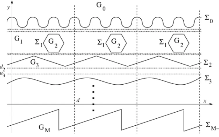
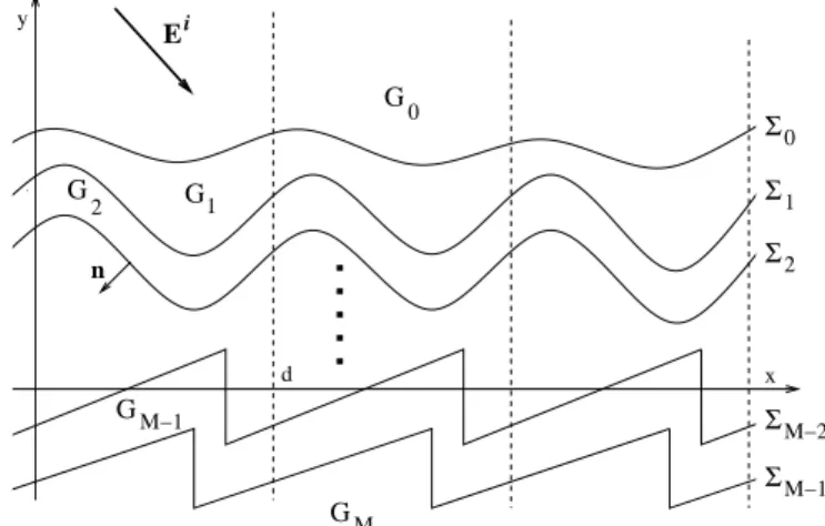
k²_±−α²n, 0≤argβn^±<π^. ^(12.15) Remark 12.2.1 The results of this section can be easily generalized to more general diffraction gratings, where the outer domains G+and G₋are bounded by surfacesΣ+andΣ−, surrounding an inner periodic grating structure. For that structure the d-periodic in x material parameters ε^(x,^y)ândµ^(x,^y)are piecewise continuous functions. Then the z-components E_zand H_zsatisfy Helmholtz equations(12.8) with variableκ²⁼ω²εµ^{, where}ε^(x,^y)ôrµ^(x,^y)are continuous, and meet the jump conditions(12.9)at any discontinuous curve ofε^(x,^y)ôrµ^(x,^y).

12.2.3 Boundary integral operators

Here we describe the application of some mathematical results on boundary integral equations to the solution of the present Helmholtz problems inG_±. Let the common boundaryΣofG₋ andG+be given by a piecewiseC²parametrization

σ(t) = (X(t),Y(t)), X(t+1) =X(t) +d,Y(t+1) =Y(t), t∈R, (12.16) i.e. the continuous functions X,Y are piecewiseC² andσ^(t1)̸=σ^(t2) ift₁̸=t₂. If the profile Σ has corners, then we suppose additionally that the angles between adjacent tangents at the corners are strictly between 0 and 2π^.

The potentials which provideα-quasi-periodic solutions of the Helmholtz equation

∆u+k²u=0 with 0≤argk²<2π ^(12.17) are based on the quasi-periodic fundamental solution of periodd

Ψk,α(P) = lim

N→∞

i 4

∑

N n=−N

H₀⁽¹⁾ (

k

√

(X−nd)²+Y² )

eⁱ^α^nd, P= (X,Y), (12.18) with the Hankel function of the first kind H₀⁽¹⁾. The series (12.18) converges uniformly over compact sets inR²\ ^∪

n∈Z{(nd,0)}if the condition k²̸=αn²=

(α⁺²πⁿ d

)2

for all n∈Z (12.19)

is satisfied. At any pointQ= (nd,0)the fundamental solution has a logarithmic singularity Ψk,α(P−Q)≍ eⁱ^α^(X−nd)^−sin(X^−nd))

2π ^log

1

|P−Q|

for P= (X,Y) near Q. Moreover, setting βⁿ ⁼^√^k²−αn² (recall that Imβⁿ ≥0) Poisson’s summation formula leads to the representation

Ψk,α(P) = lim

N→∞

i 2d

∑

N n=−N

eⁱ^αⁿ^X+i^βⁿ^|Y^| βn

, (12.20)

(14)

where in the case k<0 according to (12.7) the fundamental solution is given by (12.20) with βn=−(

k²−αn²

)_1/2 .

The single and double layer potentials are defined by Sφ^{(P) =}²^∫

Γφ^(Q)Ψk,α(P−Q)dσQ, Dφ^{(P) =}²^∫

Γφ^(Q)∂n(Q)Ψk,α(P−Q)dσQ, (12.21) whereΓis one period of the interfaceΣ, i.e. Γ={σ^(t)^:^t∈[t₀,t₀+1]}for somet₀. In (12.21) dσQdenotes the integration with respect to the arc length andn(Q)is the normal toΣatQ∈Σ pointing into G₋. Obviously, forα-quasiperiodic densitiesφ ^onΣthe potentialsSφ^,Dφ ^are α-quasiperiodic inX and do not depend on the choice ofΓ. They are solutions of the Helmholtz equation (12.17) inG_±and satisfy the radiation condition

u(x,y) =

∑

∞ n=−∞

u_neⁱ^αⁿ^x+i^βⁿ^|y|, |y| ≥H. (12.22) The potentials provide the usual representation formulas. Anyα-quasiperiodic solutionu of (12.17) inG+ satisfying (12.22) admits the representation

1 2

(S∂nu−Du)

=

{ u inG₊,

0 inG₋, (12.23)

where the normal npoints into G₋. Under the same assumptions for a function u in G₋ the representation

1 2

(Du−S∂ⁿ^u⁾⁼

{ 0 inG+,

u inG₋, (12.24)

is valid.

Restriction of the potentialsS andD to the profile curve Σare the so called boundary integral operators. The potentials provide the usual jump relations of classical potential theory.

The single layer potential is continuous acrossΣ

(Sφ⁾⁺^{(P) = (}Sφ⁾⁻^{(P) =}^Vφ^(P)^, ^(12.25) where the upper sign+resp. −denotes the limits of the potentials for points inG_± tending in non-tangential direction toP∈Σ, andV is a integral operator with logarithmic singularity

Vφ^{(P) =}²^∫

ΓΨk,α(P−Q)φ^(Q)^dσQ, P∈Σ. The double layer potential has a jump if crossingΓ:

(Dφ⁾⁺^{= (K}−I)φ^, ⁽Dφ⁾⁻^{= (K}⁺^I)φ ^(12.26) with the boundary double layer potential

Kφ^{(P) =}²^∫

Γφ^(Q)∂n(Q)Ψk,α(P−Q)dσQ+ (δ^(P)−1)φ^(P)^.

Hereδ^(P)∈(0,2),P∈Σ, denotes the ratio of the angle inG+atPandπ^{, i.e.,}δ^{(P) =}^{1 outside} corner points ofΣ. The normal derivative ofSφ^atΣexists outside corners and has the limits

(∂nSφ⁾⁺ ^{= (L}⁺^I)φ^, ⁽∂nSφ⁾⁻ ^{= (L}−I)φ^, ^(12.27)

(15)

whereLis the integral operator onΓwith the kernel∂n(P)Ψk,α(P−Q), Lφ^{(P) =}²^∫

Γφ^(Q)∂n(P)Ψk,α(P−Q)dσQ, P∈Σ. (12.28) Boundary integral methods for second order partial differential equations usually employ also normal derivatives of the double layer potential. The kernel function of this integral operator has a strong singularity of the form|P−Q|⁻²nearQ= (nd,0), and must be interpreted as hyper- singular or integro-differential operator. Since the computation of this kernel function is rather complicated and time-consuming integral methods for diffraction gratings avoid this operator.

However, in the following we need also the tangential derivative of single layer potentials

∂^t⁽^Vφ⁾^{(P) =}²∂^t^∫

ΓΨk,α(P−Q)φ^(Q)^dσQ, P∈Σ.

Interchanging differentiation and integration leads to an integral kernel with the non-integrable main singularity

t(P)·(P−Q)

|P−Q|² ,

wheret(P)denotes the tangential vector toΣatP. Therefore the tangential derivative of single layer potentials cannot be expressed as a usual integral. But it can be interpreted as the Cauchy principal value or singular integral

Jφ^{(P) =}^{2 lim}

δ→0

∫

Γ\Γ(P,δ)φ^(Q)∂t(P)Ψk,α(P−Q)dσQ=∂^t⁽^Vφ⁾^(P)^, ^(12.29) where Γ(P,δ⁾is the subarc ofΓ of length 2δ with the mid pointP. Similarly, one can define the singular integral

Hφ^{(P) =}^{2 lim}

δ→0

∫

Γ\Γ(P,δ)φ^(Q)∂t(Q)Ψk,α(P−Q)dσQ, (12.30) which by using integration by parts gives forα-quasiperiodicφ

Hφ^{(P) =}−2

∫

ΓΨk,α(P−Q)∂tφ^(Q)^dσQ=−V(

∂tφ⁾^(P)^, ^P∈Σ. (12.31) Note thatV∂tV =V J=−HV.

The integral formulation for the diffraction problems can be derived from the so-called direct or indirect approaches. The direct approach uses the representation formulas (12.23) or (12.24) together with the boundary values (12.25) and (12.26) to derive the boundary integral relations

V∂nu₊−(I+K)u₊=0 or V∂nu₋+ (I−K)u₋=0 (12.32) for quasiperiodic solutions u_± of the Helmholtz equations (12.17) in G_± satisfying (12.22).

Here the unknownsu_±and∂nu_±on the profile curveΓhave a direct physical meaning. For the indirect approach, the solution is sought as single or double layer potential with some unknown density.

An important ingredient for discussing the equivalence of integral formulations with the electromagnetic problem is the so-called "Uniqueness Theorem", which looks for conditions on Σand the wave number k such that the solution of Helmholtz equation (12.17) in G₊ or G₋ with zero boundary value onΣis identical to zero in that domain. The uniqueness of this

(16)

Dirichlet problem is equivalent to the invertibility of the single layer potential operatorV and is guaranteed by two sufficient conditions

– Imk²>0;

– the profile curveΣsatisfiesny(Q)≤0 for allQ∈Σ.

Hence, only gratings with overhanging profiles are not covered by the last condition, but it is a quite rare case that the Dirichlet problem with zero boundary data has a nontrivial solution. The only known examples, constructed in Ref. 12.15, are boundariesΣof very exotic form, which will never appear in practice.

Therefore in the following we will always assume that the "Uniqueness Theorem" is valid.

Then any quasiperiodic solution of the Helmholtz equation (12.17) inG+ orG₋ satisfying the OWC (12.22) can be uniquely determined via the representation formulas (12.23) or (12.24), respectively, or can be written as single layer potentialVφwith a quasiperiodic densityφ^{, which} belongs to some Sobolev-type space of functions given onΓ.

12.2.4 Integral equations for the in-plane case

Let us discuss examples of integral formulations for the in-plane diffraction case. Denote the z-components of the incident wave

uⁱ=

{ E_zⁱ for TE-polarization, H_zⁱ for TM-polarization.

Then for bare (one-profile) gratings the problem (12.13) (12.14) (12.11) means that one has to find a solution of

∆u_±+k²_±u_±=0 inG_±, (12.33)

satisfying continuity conditions onΣ

u₋|Σ= (u++uⁱ)|Σ, ∂n(u++uⁱ)_Σ=q∂nu₋_Σ, (12.34) and the outgoing wave condition

u₊(x,y) =

∑

∞ n=−∞

c⁺_n eⁱ⁽^αⁿ^x+^βⁿ⁺^y) fory≥H, u₋(x,y) =

∑

∞ n=−∞

c⁻_n eⁱ⁽^αⁿ^x−βⁿ⁻^y) fory≤ −H.

(12.35)

An example of the indirect approach is to look for densitiesφ+ andφ− onΓsuch that

u+=S⁺φ⁺ ^and ^u−=S⁻φ− (12.36)

satisfy (12.33-12.35), where S^± are the single layer potentials with the fundamental solution Ψk_±,α. From (12.34),(12.25) and (12.27) one derives two integral equations onΓ

V⁺φ⁺−V⁻φ− =−uⁱ

(L⁺+I)φ+−q(L⁻−I)φ− =−∂nuⁱ (12.37) HereL^±are defined by (12.28) with the kernel∂n(P)Ψk_±,α(P−Q).

(17)

The direct approach uses the relations

V⁺∂nu₊−(I+K⁺)u₊ =0,V⁻∂nu₋+ (I−K⁻)u₋=0, (12.38) following from (12.32), where the double layer potentialK^±has the kernel function∂n(Q)Ψk_±,α(P− Q). The integral equation in Ch. 4.2.3 was derived by putting (12.34) in the second equation in (12.38). Then one gets the system of integral equations

V⁺∂nu₊−(I+K⁺)u₊=0

q⁻¹V⁻∂nu₊+ (I−K⁻)u₊=−q⁻¹V⁻∂nuⁱ−(I−K⁻)uⁱ (12.39) for the unknownsu₊and∂nu₊ as functions onΓ.

Another equation system with simpler right-hand side can be obtained by the direct method if one assumes that uⁱ is a solution of∆u+k²₊u=0 inG₋ and satisfies there (12.35).

Hence, one gets additionally to (12.38)

V⁺∂nuⁱ+ (I−K⁺)uⁱ=0, leading to the relation

V⁺∂n(u₊+uⁱ)−(I+K⁺)(u₊+uⁱ) =−2uⁱ. (12.40) As before, (12.34) implies two integral equations, but now for the unknownsu₋ and∂ⁿ^u−

qV⁺∂nu₋−(I+K⁺)u₋=−2uⁱ

V⁻∂ⁿ^u−+ (I−K⁻)u₋=0 (12.41)

Note that both the direct and indirect approach lead for TE- and TM-polarization to a system of two linear integral equations with two unknowns. This is the standard approach in the boundary integral method for solving so-called transmission problems. Much effort has been spent in the theoretical and numerical analysis of different integral formulations and approximation methods for their effective solution.

It is popular in grating theory to combine the direct and indirect approaches, which results in a single integral equation for each polarization. This idea goes back to D. Maystre, who already in 1972 proposed this new approach (see Ch. 4). Take for example the representations

u₊=S⁺φ+inG₊ and u₋= 1 2

(D⁻u₋−S⁻∂nu₋)

inG₋. Then by (12.34) and (12.27)

u₋ =V⁺φ++uⁱ, ∂nu₋=q⁻¹(

(L⁺+I)φ++∂nuⁱ) such that the second relation in (12.38) implies the integral equation

(q⁻¹V⁻(I+L⁺) + (I−K⁻)V⁺)

φ+=−(

q⁻¹V⁻∂nuⁱ+ (I−K⁻)uⁱ)

(12.42) for one unknown densityφ⁺^.

Another way is to set u₊= 1

2

(S⁺∂nu₊−D⁺u₊)

inG₊ and u₋ =S⁻φ−inG₋.

(18)

In this case we derive from (12.34) and (12.27)

u₊+uⁱ=V⁻φ−, ∂n(u₊+uⁱ) =q(L⁻−I)φ−, such that (12.40) leads to the single integral equation

(qV⁺(I−L⁻) + (I+K⁺)V⁻)

φ−=2uⁱ. (12.43)

We see that the combined direct-indirect approach can lead to single integral equations for TE- and TM-problems on one-profile gratings. However, contrary to the pure direct or indirect integral method the equations contain products or compositions of boundary integral operators, which can lead to additional numerical difficulties.

12.2.5 Formulas for Rayleigh coefficients

After having solved one of the integral equation systems (12.37) or (12.41) or one of the single equations (12.42) or (12.43) it is easy to determine the complex amplitudes c^±_n of the z- components of the plane waves (12.35) reflected and transmitted by the grating—the so-called Rayleigh coefficients. We note that the functions u^±(X,Y)e⁻ⁱ^α^X for fixed ±Y ≥H, respectively, are smooth and d-periodic. Then c^±_ne^±i^βⁿ^±^Y is simply the n-th Fourier coefficient of u^±(X,Y)e⁻ⁱ^α^X, i.e.

c^±_n = e^∓i^βⁿ^±^Y d

∫ _d

0

u^±(X,Y)e⁻ⁱ^α^Xe⁻²^π^nX/ddX= e^∓i^βⁿ^±^Y d

∫ _d

0

u^±(X,Y)e⁻ⁱ^αⁿ^X dX, ±Y ≥H. The indirect approach leads to simple formulas. Supposeu_±=S^±φ±, with known den- sityφ±. Then for(X,Y) =P

c^±_n = e^∓ⁱ^βⁿ^±^Y d

∫ _d

0 S^±φ±(P)e⁻ⁱ^αⁿ^X dX

= 2 e^∓ⁱ^βⁿ^±^Y d

∫

Γφ±(Q)dσQ

∫ _d

0

e⁻ⁱ^αⁿ^X Ψk_±,α(P−Q)dX. It follows from (12.20) immediately, that withQ= (x,y)

∫ _d

0

e⁻ⁱ^αⁿ^X Ψk_±,α(P−Q)dX= i 2

e⁻ⁱ^αⁿ^x+i^βⁿ^±^|^Y⁻^y^|

βⁿ^± ^(12.44)

such that

c^±_n = i dβn^±

∫

Γe⁻ⁱ^αⁿ^x∓i^βⁿ^±^yφ±(Q)dσQ, where Q= (x,y). (12.45) Using the direct approach we find

u_±=±1 2

(S^±φ±−D^±ψ±)

with known functionsφ±,ψ±. Then c^±_n =±e^∓i^βⁿ^±^Y

2d

∫ _d

0

(S^±φ±(P)−D^±ψ±(P))

e⁻ⁱ^αⁿ^X dX

= e^∓i^βⁿ^±^Y d

∫

Γ

(φ±(Q)−ψ±(Q)∂n(Q)

)^∫ ^d

0

e⁻ⁱ^αⁿ^X Ψk_±,α(P−Q)dX dσQ.

(19)

Hence from (12.44) we get c^±_n = i

2dβⁿ^±

∫

Γ

(φ±(Q)−ψ±(Q)∂ⁿ⁾^e⁻ⁱ^αⁿ^x^∓ⁱ^βⁿ^±^y^dσQ. (12.46)

Let us apply formulas (12.45), (12.46) to the single integral equation (12.43). The Rayleigh coefficientsc⁻_n can be determined from

c⁻_n = i dβⁿ⁻

∫

Γe⁻ⁱ^αⁿ^x+i^βⁿ⁻^yφ−(Q)dσQ, (12.47) whereQ= (x,y)andφ− is the solution of (12.43). For the reflected waves we get

c⁺_n = i 2dβn⁺

∫

Γ

((q(L⁻−I)φ−−∂nuⁱ)

−(

V⁻φ−−uⁱ)

∂n

)

e⁻ⁱ^αⁿ^x−i^βⁿ⁺^ydσQ. (12.48) 12.2.6 Integral equations for the off-plane case

Now we describe the integral formulation of the conical diffraction (12.8), (12.49), (12.11) for one-profile gratings. To give the same physical dimension to the functions, we use the vacuum impedanceZ_v= (µv/εv)^1/2, whereεv,µvdenote the vacuum permittivity and permeability, respectively, and introduce B_z =Z_vH_z. Noting that γ ⁼ω⁽ε+µ+)^1/2sinϕ the jump conditions (12.9) are rewritten in the form