HAL Id: hal-00193885

HAL Id: hal-00193885

https://hal.archives-ouvertes.fr/hal-00193885v1

Preprint submitted on 4 Dec 2007 (v1), last revised 27 Mar 2009 (v2)

HAL

is a multi-disciplinary open access archive for the deposit and dissemination of sci- entific research documents, whether they are pub- lished or not. The documents may come from teaching and research institutions in France or abroad, or from public or private research centers.

L’archive ouverte pluridisciplinaire

destinée au dépôt et à la diffusion de documents scientifiques de niveau recherche, publiés ou non, émanant des établissements d’enseignement et de recherche français ou étrangers, des laboratoires publics ou privés.

Carleman estimate for elliptic operators with coefficients with jumps at an interface in arbitrary dimension and application to the null controllability of linear parabolic

equations

Jérôme Le Rousseau, Luc Robbiano

To cite this version:

Jérôme Le Rousseau, Luc Robbiano. Carleman estimate for elliptic operators with coefficients with

jumps at an interface in arbitrary dimension and application to the null controllability of linear

parabolic equations. 2007. �hal-00193885v1�

JUMPS AT AN INTERFACE IN ARBITRARY DIMENSION AND APPLICATION TO THE NULL CONTROLLABILITY OF LINEAR PARABOLIC EQUATIONS

J ´ER ˆOME LE ROUSSEAU AND LUC ROBBIANO

A. In a bounded domain of Rⁿ⁺¹, n≥2, we consider a second-order elliptic operator, A=−∂²_x0− ∇x· (c(x)∇x), where the (scalar) coefficient c(x) is piecewise smooth yet discontinuous across a smooth interface S . We prove a local Carleman estimate for A in the neighborhood of any point of the interface. The “observation”

region can be chosen independently of the sign of the jump of the coefficient c at the considered point. The derivation of this estimate relies on the separation of the problem into three microlocal regions and the Calder´on projector technique. Following the method of Lebeau and Robbiano [LR95] we then prove the null control- lability for the linear parabolic initial problem with Dirichlet boundary conditions associated to the operator

∂t− ∇x·(c(x)∇x).

Keywords: Elliptic equation; Non-smooth coefficent; Transmission problem; Carleman estimate; Microlocal analysis; Calder´on projectors; Parabolic equation; Control.

AMS 2000 subject classification: 35J15; 35S15; 35K05; 93B05; 93B07.

1. I  

The question of the null controllability of linear parabolic partial differential equations with smooth coefficients was solved in the 1990’s [LR95, FI96]. In the case of discontinuous coefficients in the principal part of the parabolic operator, the controllability issue and its dual counterpart, observability, are not fully solved yet. A result of controllability for a semi-linear heat equation with a coefficient that is discontinuous at an interface was proven in [DOP02] by means of a global Carleman observability estimate. Roughly speaking, as in the case of hyperbolic systems (see e.g. [Lio88, page 356]), the authors of [DOP02] proved their controllability result in the case where the control is supported in the region where the diffusion coefficient is the ‘lowest’. In both cases, however, the approximate controllability, and its dual counterpart, uniqueness, are true without any restriction on the monotonicity of the coefficients. It is then natural to question whether or not an observability estimate holds in the case of non-smooth coefficients and arbitrary observation location.

Recently, in the one-dimensional case, the controllability result for parabolic equations was proven for general piecewiseC¹coefficients in [BDL07a], and for coefficients with bounded variations (BV) in [Le 07], which improved the result of [FCZ02]. The proof relies on global Carleman estimates, which moreover allow to treat semilinear equations. Simultaneously, a controllability result for parabolic equations with

Date: December 4, 2007.

1

general bounded coefficients in one dimension was proven in [AE07]. The method used there to achieve null controllability is that of [LR95], which limits the field of applications to linear equations.

In the n−dimensional case, n ≥ 2, a positive answer to the controllability question was given for a class of discontinuous coefficients, with separated variables, that are smooth w.r.t. to all but one variables, which includes the case of stratified media [BDL07b]. The proof relies both on the Carleman estimates of [BDL07a, Le 07] in the one-dimensional case and the method of [LR95].

In the present article, in the case n≥2, we achieve null controllability for a linear parabolic equation in the case of a coefficient that exhibits jumps of arbitrary signs at an interface. LetΩbe a smooth bounded connected domain in Rⁿ. We consider the operator L :=∇^x·(c(x)∇^x), with possibly additional lower-order terms, and where c(x) satisfies

0<cmin≤c(x)≤cmax<∞,

to ensure uniform ellipticity for L. The coefficient c is assumed smooth apart from across an interface S , where it may jump. The interface S is the boundary of a smooth open subset Ω₁ ⋐ Ω, i.e., Ω₁ lies on one side of S . Let T >0 and set QT =(0,T )×Ω. We setΩ₂ = Ω\Ω₁. We prove the following null controllability result.

Theorem 1.1. For an arbitrary time T >0 and an arbitrary open subsetω ⊂Ωand an initial condition q₀∈L²(Ω), there exists u∈L²((0,T )×Ω) such that the solution q of

(1.1)







∂_tq−Lq=1ωu in QT,

q(t,x)=0 on (0,T )×∂Ω, q(0,x)=q0(x) inΩ,

satisfies q(T )=0 a.e. inΩ.

We follow the method of [LR95], thus proving local Carleman estimates for an elliptic operator associ- ated to the considered parabolic problem: we introduce the elliptic operator A :=−∂²_x0−L. The variable x0is an additional variables in (0,X0), for some X0 >0. We provide such a local Carleman estimate for the operator A in a small neighborhood V of a point (y0,y) of (0,X0)×S with an “observation” on one side of S , independently of the sign of the jump of c at (y0,y). We hence treat all possible cases including the case that can be treated more classically as mentioned above, for which the “observation” is supported in the region where the diffusion coefficient is the ‘lowest’ [DOP02].

We denote by (., .) the inner product on L²((0,X₀)×Ω) and byk.k⁰the induced norm. In the present article, we shall make use of techniques from the semi-classical analysis of pseudodifferential operators (ψDOs) [Mar02]. With h as the small parameter, we set D = ^h

i∂. Accordingly, we shall use the semi-classical Sobolev normkfk²k :=P

|α|≤kkD^α_x0,xfk²0, k∈N.

The Carleman estimate we aim at proving is of the form

hke^ϕ/hwk²0+h³ke^ϕ/h∇^x0,xwk²0 ≤Ch⁴ke^ϕ/hfk²0, Aw= f, h>0,

for h sufficiently small and supp(w)⊂V, when w is smooth on both sides of the interface, with w and c∂nw continuous across S (∂nis the normal derivative at S ), which implies Aw∈L²((0,X0)×Ω).

The sign of∂nϕat the interface locates the side of the interface on which the “observation” takes place (see Section 2 for the application of the local Carleman estimate). To achieve such a Carleman estimate we follow the method of [LR97], in the spirit of the work of [Bel03]. In particular, we separate the interface problem into three microlocal regions for which partial Carleman estimates are obtained. In some of these regions we make use of the Calder´on-projector technique.

With this local Carleman estimate at the interface, we can then prove an interpolation inequality that first yields an estimation of the loss of orthogonality for the eigenfunctionsφj(x), j∈N, of the operator L, with Dirichlet boundary conditions, when these eigenfunctions are restricted toω. We denote byµj, j∈N, the associated eigenvalues, sorted in an increasing sequence.

Theorem 1.2. For any (a_j)_j∈N⊂C we have:

X

µ_j≤µ

|aj|²≤Ce^C√µ Z

ω

X

µ_j≤µ

ajφj(x)

2

dx, µ >0.

(1.2)

Following [LR95], this estimation then yields a construction of the control function u(t,x) in (1.1), by sequentially acting on a finite yet increasing number of eigenspaces, and we hence obtain the result of Theorem 1.1. We refer the reader to [LR95] or [LZ98, Section 5, Proposition 2] for the details.

The reader will observe that the proof of the Carleman estimate can be adapted to other elliptic operators with non-smooth coefficients across an interface. Beyond the controllability result of interest in this arti- cle, such Carleman estimates have a wide range of applications, including unique continuation properties ([H¨or63, Zui83, H¨or85a]. See Remark 2.8 for further details.

The result of this article opens perspectives for future research towards the null controllability of semi- linear parabolic equations with non smooth coefficient in space dimension n ≥2 and towards more com- plicated geometrical situations, for instance in the case of coefficients with singularities that do not lie on a smooth interface.

In this article, when the constant C is used, it refers to a constant that is independent of the semi-classical parameter h. Its value may however change from one line to another. If we want to keep track of the value of a constant we shall use another letter. We shall use of the notationhηi:=(1+|η|²)¹². Let us now introduce semi-classicalψDOs. We denote by S^m(Rⁿ⁺¹×Rⁿ⁺¹), S^mfor short, the space of smooth functions a(z, ζ,h), defined for h∈(0,h0] for some h0>0, that satisfy the following property: for allα,βmulti-indices, there exists Cα,β≥0, such that

∂^α_z∂^β_ζa(z, ζ,h)

≤Cα,βhζi^m−|β|, z∈Rⁿ⁺¹, ζ∈Rⁿ⁺¹, h∈(0,h0].

Then, for all sequence am−j ∈ S^m−j, j∈ N, there exists a symbol a∈ S^msuch that a ∼P

jh^jam−j, in the sense that a−P

j<Nh^jam−j∈h^NS^m−N(see for instance [Mar02, Proposition 2.3.2] or [H¨or85b, Proposition 18.1.3]), with amas principal symbol. We defineΨ^mas the space ofψDOs A=Op(a), for a∈S^m, formally

defined by

A u(z)=(2πh)⁻⁽ⁿ⁺¹⁾ Ï

e^{ihz−t,ζi/h}a(z, ζ,h) u(t) dt dζ, u∈S ^′(Rⁿ⁺¹).

We shall denote the principal symbol ambyσ(A). We shall use techniques of pseudodifferential calculus in this article, such as construction of parametrices, composition formula, formula for the symbol of the adjoint operator, etc. We refer the reader to [Tay81, H¨or85b, Mar02]. In the main text the variable z will be (x₀,x) andζ =(ξ₀, ξ).

We now introduce tangential symbols and associated operators. We set z =(z^′,zn), z^′ =(z0, . . . ,zn−1) andζ^′ = (ζ0, . . . , ζn−1) accordingly. We denote by S^m

T(Rⁿ⁺¹ ×Rⁿ), S^m

T for short, the space of smooth functions b(z, ζ^′,h), defined for h∈(0,h0] for some h0 >0, that satisfy the following property: for allα,β multi-indices, there exists Cα,β≥0, such that

∂^α_z∂^β_ζ′b(z, ζ^′,h)

≤Cα,βhζ^′i^m−|β|, z∈Rⁿ⁺¹, ζ^′∈Rⁿ, h∈(0,h₀].

As above, for all sequence bm−j∈S^m−j

T , j∈N, there exists a symbol b∈S^m

T such that b∼P

jh^jbm−j, in the sense that b−P

j<Nh^jbm−j∈h^NS^m−N

T , with bmas principal symbol. We defineΨ^m

T as the space of tangential ψDOs B =op(b) (observe the notation we adopt is different from above to avoid confusion), for b ∈S^m

T, formally defined by

B u(z)=(2πh)⁻ⁿ Ï

e^{ihz′−t′,ζ′i/h}b(z, ζ^′,h) u(t^′,z_n) dt^′dζ^′, u∈S ^′(Rⁿ⁺¹).

We shall also denote the principal symbol bmbyσ(B). In the case where the symbol is polynomial inζ^′ and h, we shall denote the space of associated tangential differential operators byD^m_T. We shall denote by Λ^sthe tangentialψDO whose symbol ishζ^′i^s. The composition formula for tangential symbols, b ∈S^m

T, b^′∈S^m′

T, is given by

(b #_Tb^′)(z, ζ^′)=(2πh)⁻ⁿ Ï

e^{−iht′,τ′i)/h}b(z, ζ^′+τ^′,h) b^′(z^′+t^′,zn, ζ^′,h) dt^′dτ^′ (1.3)

= X

|α|≤M

(−ih)^|α|

α! ∂^α_ζ′b(z, ζ^′,h)∂^α_z′b^′(z, ζ^′,h) +(−ih)^M+1

(2πh)ⁿ X

|α|=M+1 1

Z

0

(M+1)(1−s)^M α!

Ï

e^{−iht′,τ′i)/h}∂^α_ζ′b(z, ζ^′+τ^′,h)∂^α_z′b^′(z^′+st^′,zn, ζ^′,h) dt^′dτ^′ds,

and yields a tangential symbol in S^m+m′

T . In the main text the variable z will be (x0,x^′,xn) andζ^′=(ξ0, ξ^′).

Following [LR95, LR97], we shall denote by (., .)₀the inner product for functions defined on{xn =0}, i.e., ( f,g)₀ := ^Îf (x0,x^′) g(x0,x^′) dx0 dx^′. The induced norm is denoted by|.|0, i.e.,|f|²0 = ( f,f )₀. For s∈R we introduce|f|s:=|Λ^sf|0.

The outline of the article is as follows. In section 2, we prove the announced local Carleman estimate at the interface for the elliptic operator A. In Section 3, we prove the interpolation inequality that implies (1.2). The controllability result then follows from [LR95].

2. LC    

In the neighborhood of a point (y0,y) of (0,X0)×S , we denote by xn the variable that is normal to the interface S and by x^′the remaining spacial variables, i.e., x =(x^′,xn). In particular y =(y^′,0). The transmission conditions at the interface we shall consider are

∀x₀,x^′, w|^xn=0⁻ =w|^xn=0⁺+θ, c∂_xnw|^xn=0⁻ =c∂_xnw|^xn=0⁺+ Θ, (TC)

i.e., the continuity of w at the interface as well as the continuity of the normal flux, modulo some error terms θandΘ. Such error terms will be usefull in Section 3 where the Carleman estimate proven in this section is used to achieve the null controllabiltity result of Theorem 1.1.

In a sufficiently small neighborhood V⊂Rⁿof (y0,y), we place ourselves in normal geodesic coordinates (w.r.t. to the spacial variables x). For convenience, we shall take the neighborhood V of the form (y0 − ε,y0+ε)×Vy^′×(−ε, ε), where Vy^′ is a sufficiently small neighborhood of y^′. In such coordinate system, the principal part of the differential operator A takes the following form [H¨or85b, Appendix C.5] on both sides of the interface:

A2=−∂²_x0−c(x)

∂²_xn−r(x, ∂x^′/i) ,

with r(x, ξ^′) a xn-family of second-order polynomials inξ^′that satisfy

r(x, ξ^′)∈R, and C1|ξ^′|²≤r(x, ξ^′)≤C2|ξ^′|², x∈Vy^′×(−ε, ε), ξ^′∈Rⁿ, (2.1)

for some 0<C₁≤C₂ <∞. Note that the transmission conditions (TC) remain unchanged in this change of variables.

We set

Rⁿ₋⁺¹={(x₀,x),x_n<0}, Rⁿ₋⁺¹={(x₀,x),x_n≤0}, Rⁿ+⁺¹={(x₀,x),x_n>0}, Rⁿ+⁺¹={(x₀,x),x_n≥0}, V^g=V∩Rⁿ₋⁺¹, V^d =V∩Rⁿ+⁺¹, K^g=V^g, K^d =V^d, and K=V.

We denote byCc^∞(K^g) (resp.Cc^∞(K^d)) the space of functions that areC^∞in Rⁿ₋⁺¹(resp. Rⁿ+⁺¹) with support in K^g(resp. K^d).

We letϕbe a (weight) function in all variables. We shall “observe” the solution of the elliptic equation Aw= f on the side xn >0 and thus choose∂x_nϕ(x0,x^′,xn=0^±)>0. We shall consider three cases in order to treat the general case:

Case 1: c(y^′,yn =0⁻)<c(y^′,yn =0⁺), Case 2: c(y^′,yn =0⁻)=c(y^′,yn =0⁺), Case 3: c(y^′,yn =0⁻)>c(y^′,yn =0⁺).

Recall that Case 3 is the case for which controllability and global Carleman estimates were obtained in [DOP02].

On both sides of S we define Aϕ =h²e^ϕ/hA2e^−ϕ/h. Considered as a semi-classical differential operator we denote by aϕits principal symbol, which is given by

aϕ=(ξ0+i∂x₀ϕ)²+c(x)

(ξn+i∂x_nϕ)²+r(x, ξ^′+i∂x^′ϕ) .

We make the following assumption.

Assumption 2.1. The weight functionϕ(x0,x) is inC(V) andϕ|_Rⁿ⁺¹

∓ ∈C^∞(K^g/d) and satisfies|∇^(x0,x)ϕ|>0 in V. We assume

∀x0,x^′, ∂x_nϕ(x0,x^′,xn=0^±)>0, ∂x_nϕ(x0,x^′,xn=0⁺)−∂x_nϕ(x0,x^′,xn=0⁻)≥C>0, (2.2) (c∂x_nϕ)(x0,x^′,xn=0⁺)−(c∂x_nϕ)(x0,x^′,xn=0⁻)≥0.

The functionϕsatisfies the sub-ellipticity condition

∀(x0,x, ξ0, ξ)∈K^g/d×Rⁿ⁺¹, aϕ(x0,x, ξ0, ξ)=0 ⇒ {Re aϕ,Im aϕ}(x, ξ)>0.

(2.3)

Case 1: The neighborhood V is chosen sufficiently small such that

c(x^′,xn=0⁺)−c(x^′,xn=0⁻)≥C>0, x^′∈Vy^′. Moreover we assume

(2.4) ∀x₀,x^′, ∂_xnϕ(x₀,x^′,x_n=0⁺)2

− ∂_xnϕ(x₀,x^′,x_n=0⁻)2

− ∂_x0ϕ(x₀,x^′,x_n=0)2 1

c(x^′,xn =0⁻)− 1 c(x^′,xn=0⁺)

!

≥C>0.

Case 2: The neighborhood V is chosen sufficiently small such that|c(x^′,x_n =0⁻)−c(x^′,x_n =0⁺)|is itself sufficiently small.

Case 3: The neighborhood V is chosen sufficiently small such that

c(x^′,xn=0⁺)−c(x^′,xn=0⁻)≤ −C<0, x^′∈Vy^′. Moreover we assume

(2.5) ∀x0,x^′, (c(x^′,xn=0⁺))²

c(x^′,xn=0⁻) ∂x_nϕ(x0,x^′,xn =0⁺)²

−c(x^′,xn=0⁻) r(x^′,xn=0, ∂x^′ϕ(x0,x^′,xn=0))≥K, where K is some positive constant and

(2.6) ∀x0,x^′, C1 1−c(x^′,xn=0⁺) c(x^′,xn=0⁻)

!  1

(c∂x_nϕ)(x0,x^′,xn =0⁻)2 − 1

(c∂x_nϕ)(x0,x^′,xn=0⁺)2





−C²₂(∂_x0ϕ)²(x0,x^′,xn=0) 1

c(∂x_nϕ)²(x0,x^′,xn=0⁻)− 1

c(∂x_nϕ)²(x0,x^′,xn=0⁺)

!2 _x

n=0⁺

≥0, where C1and C2are the constants in (2.1).

Note thatϕis chosen continuous across the interface. In particular, we have

∂x₀ϕ|^xn=0⁻ =∂x₀ϕ|^xn=0⁺, ∂x^′ϕ|^xn=0⁻=∂x^′ϕ|^xn=0⁺, which we shall simply write∂_x0ϕ|^xn=0⁺and∂_x′ϕ|^xn=0⁺respectively in the sequel.

The conditions we impose on the weight functionϕwill make sense in the course of the proof of Propo- sition 2.7 below. In Section 3 we shall construct a weight function that statisfies the properties listed in Assumption 2.1.

From the assumption made on the weight functionϕwe shall obtain the following local Carleman esti- mate.

Theorem 2.2. Let the coefficient c(x) satisfy Cases 1, 2 or 3. With the weight functionϕsatisfying Assump- tion 2.1, there exist C >0 and h0>0 such that

(2.7) hke^ϕ/hwk²0+h³ke^ϕ/h∇^x0,xwk²0+h|e^ϕ/hw|^xn=0^±|²0+h³|e^ϕ/h∂x₀,x^′w|^xn=0^±|²0+h³|e^ϕ/h∂x_nw|^xn=0^±|²0

≤C

h⁴ke^ϕ/hfk²0+h|e^ϕ/hθ|²0+h³|e^ϕ/h∂x₀,x^′θ|²0+h³|e^ϕ/hΘ|²0

, 0<h≤h0, for w satisfying (TC), w|_Rⁿ⁺¹

∓ ∈Cc^∞(K^g/d) and A₂w= f .

Remark 2.3. This Carleman estimate yields the same estimate for the operator A making use of the insen- sitivity of such estimates to changes of variables and to additional lower-order terms.

The remainder of this section is devoted to the proof of Theorem 2.2.

2.1. Preliminaries. We assume that the function w satisfies (TC) and A2w = f . Following [Bel03], we shall consider the transmission problem as a system of two equations on V^dcoupled at the boundary xn=0⁺. We thus make the change of variables xnto−xnin V^g. This yields the following system on V^d:



(−c^g1(x)∂²_x0−(∂²_xn−r^g(x, ∂x^′/i))) w^g=F^g = ¹

c^g(x)f^g, (−c^d1(x)∂²_x0−(∂²_xn−r^d(x, ∂x^′/i))) w^d=F^d = ¹

c^d(x)f^d, (2.8)

with

w^g|^xn=0⁺=w^d|^xn=0⁺+θ, c^g∂x_nw^g|^xn=0⁺+c^d∂x_nw^d|^xn=0⁺ = Θ, (TC^∗)

where for a functionψdefined in V, we setψ^d :=ψ|^Vdandψ^g(x^′,x_n)=ψ(x^′,−x_n) for x_n>0. In particular, we have r^g(x, ∂_x′/i) = r(x^′,−x_n, ∂_x′/i), and r^d(x, ∂_x′/i) = r(x, ∂_x′/i) for x_n > 0. If there is no possible confusion, we shall now writeψ=t(ψ^g, ψ^d). From Assumption 2.1 we have

∂_xnϕ^g(x0,x^′,xn=0)<0, ∂_xnϕ^d(x0,x^′,xn=0)>0, (2.9)

and

c^g∂_xnϕ^g(x₀,x^′,x_n=0)+c^d∂_xnϕ^d(x₀,x^′,x_n=0)≥0.

(2.10)

Observe also that condition (2.3) is preserved since{Re aϕ,Im aϕ}is invariant under a change of variables [H¨or63, Section 8.1, page 186].

We denote by p^g/d the symbols of the operators acting on w^g/d in (2.8). We set P(x0,x,Dx₀,Dx) := Op(diag(p^g,p^d)) and Φ := diag(ϕ^g, ϕ^d). We set v = t(v^g,v^d). For v = e^Φ/hw, the entries of v satisfy the following boundary condition

v^g|^xn=0⁺=v^d|^xn=0⁺+θ_ϕ, c^g(Dxn+i∂_xnϕ^g)v^g|^xn=0⁺+c^d(Dxn+i∂_xnϕ^d)v^d|^xn=0⁺= Θ_ϕ, (TCϕ)

where

θ_ϕ=e^ϕ/h|^xn=0⁺θ and Θ_ϕ=h

ie^ϕ/h|^xn=0⁺Θ. (2.11)

We define the following conjugated operator Pϕ =h²e^Φ/hPe^−Φ/h, which we shall, in the sequel, treat as a second-order semi-classical differential operator, with h as the small parameter. The principal symbol of Pϕ

is given by

pϕ(x0,x, ξ₀, ξ^′, ξ_n)=diag(p^gϕ(x0,x, ξ₀, ξ^′, ξ_n),p^d_ϕ(x0,x, ξ₀, ξ^′, ξ_n)), with

p^g_ϕ^/d(x₀,x, ξ₀, ξ^′, ξ_n)= 1

c^g/d(ξ₀+i∂_x0ϕ^g/d)²+(ξ_n+i∂_xnϕ^g/d)²+r^g/d(x, ξ^′+i∂_x′ϕ^g/d).

For the sake of concision, we shall often omit the time and spacial variables in the functions c^g/d andϕ^g/d, as we have just done, when there is no possible confusion. Separating the real and imaginary parts of the principal symbol, we write p^g_ϕ^/d =˜q^g₂^/d+i ˜q^g₁^/d, and following [LR95] we set

˜q^g₂^/d=ξ_n²+q^g₂^/d, ˜q^g₁^/d=2∂x_nϕ^g/dξn+2q^g₁^/d, with

q^g₂^/d(x0,x, ξ0, ξ^′)=−

∂x_nϕ^g/d2

+ 1 c^g/d

ξ₀²−

∂x₀ϕ^g/d2

+r^g/d(x, ξ^′)−r^g/d(x, ∂x^′ϕ^g/d), q^g₁^/d(x₀,x, ξ₀, ξ^′)= 1

c^g/d∂_x0ϕ^g/dξ₀+˜r^g/d(x, ξ^′, ∂_x′ϕ^g/d),

where ˜r^g/d(x, ξ^′, η^′) are the symmetric bilinear forms inξ^′,η^′associated to the real quadratic forms r^g/d(x, ξ^′).

2.2. Signs of the imaginary part of the two roots of p_ϕ^g/d. At x_n=0⁺, the polynomials (inξ_n) p^g_ϕ^/d(x₀,x, ξ₀, ξ^′, ξ_n) have two complex roots. Depending on the signs of the imaginary parts of the two roots of the two poly- nomials, we shall adopt different strategies for the proof of partial Carleman estimates. By “partial” we actually mean that the resulting estimate will only hold in some microlocal region. Once collected together, the partial estimates will yield the result of Theorem 2.2.

Following [LR97], we set

µ^g/d(x₀,x, ξ₀, ξ^′) :=q^g₂^/d(x₀,x, ξ₀, ξ^′)+

q^g₁^/d(x₀,x, ξ₀, ξ^′)2

∂x_nϕ^g/d2 , (2.12)

and define

E^g/d,+:={(x0,x, ξ0, ξ^′)∈V^d×Rⁿ; µ^g/d(x0,x, ξ0, ξ^′)>0}, E^g/d,−:={(x0,x, ξ0, ξ^′)∈V^d×Rⁿ; µ^g/d(x0,x, ξ0, ξ^′)<0}, Z ^g/d :={(x0,x, ξ₀, ξ^′)∈V^d×Rⁿ; µ^g/d(x0,x, ξ₀, ξ^′)=0}.

Remark 2.4. The regionsE^g/d,−andZ^g/d are bounded. Hence, for|(ξ0, ξ^′)|sufficiently large, say|(ξ0, ξ^′)|>

R, then (x0,x, ξ0, ξ^′)∈E^g,+∩E^d,+, with dist((x0,x, ξ0, ξ^′),Z^g/d)≥C>0.

The following lemma is proven in [LR97, proof of Lemma 3].

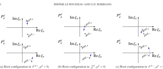
Lemma 2.5. In the region E^g/d,+, the polynomials p^g_ϕ^/d have two distinct roots ρ^g/d,+and ρ^g/d,− that satisfy Imρ^g/d,+ >0 and Imρ^g/d,− <0. In the regionE^g/d,−, the imaginary parts of the two roots have the same sign as that of−∂x_nϕ^g/d. InZ ^g/d, one of the roots is real.

Hence, for the polynomial p^d_ϕ, for|(ξ₀, ξ^′)| >R, there are two roots,ρ^d,+andρ^d,−with Imρ^d,+ >0 and Imρ^d,− <0. As the value ofµ^d decreases, the rootρ^d,+moves towards the real axis, and crosses it in the regionZ^d. In the regionE^d,−the two roots both have negative imaginary parts.

For the polynomial p^g_ϕ, for|(ξ0, ξ^′)|>R, there are two roots,ρ^g,+andρ^g,−with Imρ^g,+>0 and Imρ^g,−<

0. As the value ofµ^gdecreases, the rootρ^g,−moves towards the real axis, and crosses it in the regionZ^g. In the regionE^g,−the two roots both have positive imaginary parts. The “motion” of the roots of p^gϕand p^d_ϕ is illustrated in Figure 1.

Remark 2.6. From the proof of Lemma 3 in [LR97], we see thatµ^g/d ≥ C > 0 is equivalent to having Imρ^g/d,+≥C^′>0 and Imρ^g/d,−≤ −C^′.

With the choice of weight functionϕmade in Assumption 2.1 we have the following proposition.

Proposition 2.7. The properties of the weight functionϕimplyE^d,+⊂E^g,+, and dist(E^d,+,Z^g)≥C>0, if the neighborhood Vyof y is chosen sufficiently small.

The result of the proposition implies that the rootρ^d,+crosses the real axis before the rootρ^g,+does, asµ^d decreases from positive to negative values. This is illustrated in Figure 1. We enforce this root configuration because of the techniques we shall use to prove partial Carleman estimates.

In the case where the roots of the polynomial are separated by the real axis, or in the case where they are both in the lower open half plane, we can apply the Calder´on-projector technique to the associated differential operator. The first case occurs for P^g_ϕ^/d in regionsE^g/d,+. The second case can only occur for P^d_ϕ in the regionE^d,−. In such regions, the Calder´on-projector technique in fact yields an additional boundary condition at xn=0⁺.

In fact, the choice of weight functionϕwe have made excludes the situation in which Imρ^g,± >0 and the rootρ^d,+may cross the real axis. In such a case, the Calder´on projector technique cannot be used for