Those singularities coincide with discontinuities of the optimal (or at least, extreme) control, called linkages. Applications of the Galois differential theory methods are rare in the context of optimal control.
Controllability
Intuitively, this is not the case in systems that are affine with control, since the drift can be too strong relative to the control and thus disable control. When the offset is reasonable, i.e. does not take the system to infinity, we can imagine that control can be achieved.
Geometric optimal control
The maximization condition allows us to compute the optimal control, moreover, whose maximum is in the interior of the set U we have. In this chapter we are mainly interested in the minimal time management of mechanical systems, namely mold systems.
Singularities of minimum time control for mechanical systems
Setting
Since we are interested in the behavior of the extreme current and its singularity, we can drop the parameter ε and consider the control in the uniform Euclidean sphere. The extremum lying from Σ is the integral curve of the maximized Hamiltonian Hmaxpzq “ H0pzq `a.
Stratification of the extremal flow
It then becomes clear that the flow of the nilpotent approximation is smooth outside Ss. Recall that the Jacobian of the vector field has a convenient spectrum on N: a 6-dimensional kernel, and two eigenspaces with. We will prove that in a neighborhood Oz¯´ of ¯z´, the situation is symmetric around ¯z`, and an extremal in Σ spends 0 time t.
Note now that zpt, z0q "zpt´t10, zpt10, z0qq and we use the regularity of the system when the singular locus is not crossed to.
Regular-singular transition
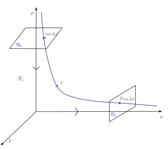
Then T is a smooth function in pω0lnω0, ω0, ξ0q since there exist smooth functions R and X defined on a neighborhood of t0u ˆ t0u ˆD such that. When one crosses Σ, the determinantad´bc becomes 0, and one indeed gets singularities of the form "zlnz". By the above remark, there exists Y8 a smooth vector field on O such that W " Y8`R8 where R8 is a smooth function with zero infinite radius along D.
This can be achieved using the method of the path: Instead of looking for a diffeomorphism sending Y0 :" Y onY1 :"Y8`R8, we search for a one-parameter family (path) of diffeomorphism (gt) such.
Application to mechanical systems
The switch corresponds to a momentary rotation of the steering angle π (the so-called π-singularity). Let q P M “ R2zt´µ,1´µu be the position vector and consider µ the mass ratio of the two primary elements. The controlled circular constrained three-body problem is a reduction (CRTBP) where the two primary bodies are in circular motion about their center of mass.
It remains to study the zeros in the adjoint statepv to access the switching times.
Conclusion and perspectives
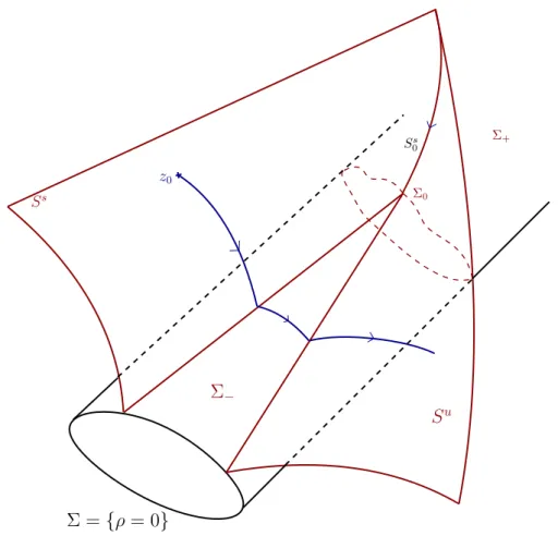
Thus the projection of the singular site Σ becomes of codimension one and the extremals will generically cross it. We also give the regularity of the extreme current around the singular point and describe the jump on the control in the switching time. In this chapter, we give a detailed description of the behavior of the extreme flow around the singularity.
By Pontrjagin's maximum principle, optimal trajectories are the projection of integral curves of the maximized Hamiltonian system defined on the cotangent bundle of M by .
The bifurcation formulation
The case Σ ´
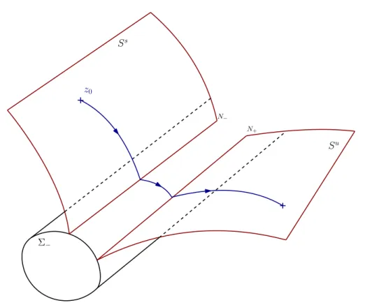
Recall that for the sake of clarity, we will work in a neighborhood of 0, taking into account that we do not lose generality (and the result holds for every point). In a neighborhood Oz¯ with z¯PΣ´, existence and uniqueness, all extremes are noise, with at most one key. Su) is the codimension—a submanifold of the initial conditions leading to the switching surface (respectively at negative times), S0 “ O¯zzpSs YΣq.
In [22] the authors also studied the regular-singular transition between the strata and showed log-type singularities.
The case Σ `
Despite the absence of a switch, there is a singular current within Σ` as shown in [22], but the singular extremum lying in Σ` cannot be optimal under Goh's condition, [20].
The bifurcation α “ 0: case Σ 0
In the process of proving Theorem 2.2, we obtained a clear description of the singular flow around a point Σ0. In the direction of u, at each of these points is a stable one-dimensional manifold. In the first alternative, the extremum reaches the singular locus at the equilibrium point at timeρdt, and we have θp¯tq ´φp¯tq “ π{2: the control is continuous when the connection to the singular flow occurs.
The dynamics is in fact structurally stable and the whole situation is contained in the nilpotent case Σ0.
Conclusion
Since we have the existence and uniqueness of the solutions of the extremal system, we would like to use Philipp's theorem to obtain a global result about their optimality, see [24]. An extension of the smooth case method that uses the Poincaré-Cartan integral invariant, see [4], is more easily generalized to non-smooth cases and has been used to prove local optimality for L1 minimization of mechanical systems, for example in [ 19 ]. We use a similar technique to prove Theorem 3.2, with one of the main differences being the type of singularity: the L1-minimization of the control produces singularities of codimension one, and the extremal current is the concatenation of the current of two regular Hamiltonians.
The proof consists in building a Lagrangian manifold, and propagating into the extreme current, then one can prove that the projection is invertible on this manifold: this makes it possible to lift all the allowed trajectories with the same endpoints to the cotangent bundle, and one can compare their cost using the Poincaré-Cartan invariant with that of the reference extremals.
Our setting
The p2q assumption provides disconjugation along the reference extremum and can be verified by a simple numerical test. We will extend this proof to the non-smooth case of our control systems with minimum time affinity. According to Theorem 2.1 in Chapter II, we know the extreme current with isPC8 in the neighborhood of Σ´.
Write the extreme current as the integral of the regularized vector field (see Chapter I) X: zpt¯pz0q, z0q “ ş`8.
Proof of theorem 3.2
It means that, in a neighborhood of ¯z, every extremum passes transversally through πpΣ1q: limiting S0 if necessary, every extremum fromS0 passes transversally through πpΣ1q, and the projection defines a continuous bijection on S1YS2, even even a homeomorphism if we limit ourselves to a compact neighborhood of the reference extremum. Now, let us prove that our extremal reference ¯z " px, ¯ pq¯ minimizes the final time between all adjacent curves C1 with the same endpoints. To extend the result to all admissible adjacent curves, consider a curve such ˜x with the same endpoints and denote ˜u its associated control.
Take a C1 curve x in a small enough neighborhood of ˜x in the W1,8 topology (allowable curves are absolutely continuous).
Regularity of the field of extremal
First case In the vicinity of px0,p¯0q PSs, the extreme flow, as well as F, is smooth. In such a neighborhood, we only have PC1 regularity for G, and we need a weaker inverse function theorem. In case it is globally optimal, the value function is justSpxfq " tfpxfq, the last time for extremal.
Otherwise, we have Spxfq ď tf and we only have the regularity PC1 for the upper bound function on the value function: the finite time of the extreme trajectories.
Conclusion and perspectives
Integrability of Hamiltonian systems and optimal control
If n“2,Upqq “ ´}q}1 (}.} is the Euclidean norm), H defines the famous Kepler problem (we saw the controlled version in example 1.1), which describes the reduction of the motion of two bodies which attract others by the Newtonian gravity in the plane. We now recall some facts of the theory of integrable systems, starting with the definition of integrability. The first, obvious one, is that every integral curve is contained in one of the n-dimensional manifolds Mc “tpf1.
One of the first examples of proof of non-integrability is Poincaré's famous work in [50] for the three-body problem.
Introduction to Galois Differential Theory
The Galois group being a closed subgroup of Glnpk0q for a linear differential equation of order, it also has a Lie group structure. The local Galois differential group in x is the Galois group over the basic field “Cxptzuq: the field of meromorphic functions in a neighborhood ofx. To explore the connection between the monodrome group and the Galois group, we need the notion of Fuchsian equations.
Then Π is dense for the Zariski topology in the Galois group of the Picard-Vessiot expansion pEq over the basic field of rational functions: Π“GalpAq.
Integrability and its obstructions in Hamiltonian systems coming
Setting
The next fundamental result is Pontrjagin Maximum Principle [51] (see [4] for a modern presentation). i) px, pq is a solution of the Hamiltonian system associated with Hp¨,¨, uptqq: x9 “ BH. As a consequence of the maximization condition, the pseudo-Hamiltonian is evaluated along an extremal constant. The Hamiltonian is defined on the cotangent bundle of the original phase space, and thus the dimension is doubled.
It is a complex complex manifold (with local Darboux coordinates, pq outside the singular hypersurface 1r2 “0), on which H lies meromorphically, even rationally, since. 4.2.7) The Hamiltonian H has four degrees of freedom, so (see [5]) the meromorphic Liouville integrability of H over M would imply that there would exist three independent first integrals, apart from H itself, almost everywhere in M.
Proof of Theorem 4.9
It is sufficient to find an obstacle in this modified tense, as explained at the end of the proof. Using the expression of the first integralC and of the vector field we derive x3px1q. Moralès–Ramis theorem provides necessary conditions for Liouville integrability in terms of the Galois group of this linear differential system over the basis field of meromorphic functions on Γ.
Since the Picard-Vessiot field is generated by all components of the solutions, the Picard-Vessiot field K is generated by the normal variational equation.
Conclusion and perspectives
It can be understood as follows: The Galois group contains the monodrome group, which is the group obtained by analytic continuity around the singularities of the differential equation. If this set is large enough, integrability cannot occur, and this is a consequence of the optimization procedure (ie, P.M.P.). It becomes interesting to look at the problem from the perspective of the perturbation theory of Kolmogorov, Arnold and Mother, see the annex of [5], or [30] for a modern review on KAM theory.
The persistence of KAM tori under this perturbation would then imply the non-geodesic convexity of the minimum-time Kepler problem, as in the case of mean energy.


