P± density functions of the gray levelI on-road (+) and off-road (-) Q± density functions of the varianceOff-road (+) and off-road. In this chapter, we present a brief state-of-the-art for active contouring and path extraction.
Active Contours
The GVF is calculated as the diffusion of the gradient vectors of the edge map derived from the image. 1.3) Thus, the external force of the evolution equation in the snake model is replaced by the GVF field.
Road Extraction
In the final stage, the paths are extracted by a simple threshold applied to the response of the morphological operators. The specific characteristics of the road network in the image are described by the data term.
Conclusion
This chapter presents the phase-field higher-order active contour (HOAC) framework for image segmentation. Later, 'phase fields' were introduced for region modeling in (Rochery et al., 2005a), where HOACs are reformulated as (non-local) phase field models.
A General Framework for Image Segmentation
They are thus more robust and can be generically initialized, i.e. automatically, and thus outperform conventional active contours. From this formulation, the optimal image partitioning can be calculated by finding the region R with the maximum posterior probability.
Summary of Higher-Order Active Contours and Phase Fields
The initial value of the phase field function is set everywhere in the image domain to a suitable value z (a constant depending on the mathematical definition of the model). Due to the above advantages, phase field representation and phase field modeling are the preferred methodology in this thesis.

Stability Analysis of the Standard HOAC Total Prior Model
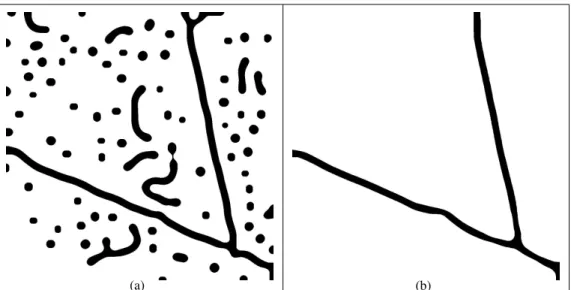
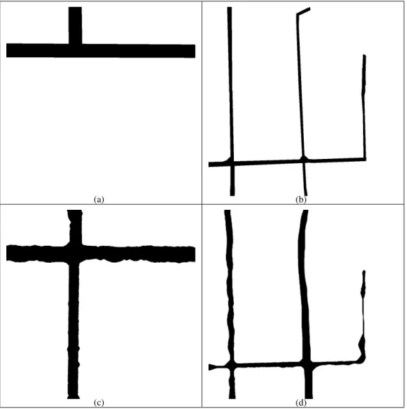
According to the definition of the interaction function Ψ (equation (2.5)), the first integral is equal to The solid curve represents the extremum as a local minimum, i.e. the second constraint in equation (2.19b) is satisfied; while the dashed curve represents the extremum as a local maximum, i.e. the second constraint is not met. The straight bars disappear one by one due to the weak force of the squared energy.

Overall Model for Linear Network Extraction
In the experimental results on the real images that we will show later, ˆβ is set so that each unit length of a straight beam adds a small but positive amount to the total energy because the data can indicate the preferred regions. Because in the edge-based data expression, the local descriptor, such as the gradient vector, considers neighborhoods that are very small compared to the size of the image, the algorithm can easily get trapped in one of the many local minima of the energy. There are also certain intuitions that can be used to specify order-of-magnitude settings for this parameter: the forces due to the prior term should not be much larger than or much smaller than the forces due to the data term, otherwise the prior will dominate in one case and have little effect in the second.
Conclusion
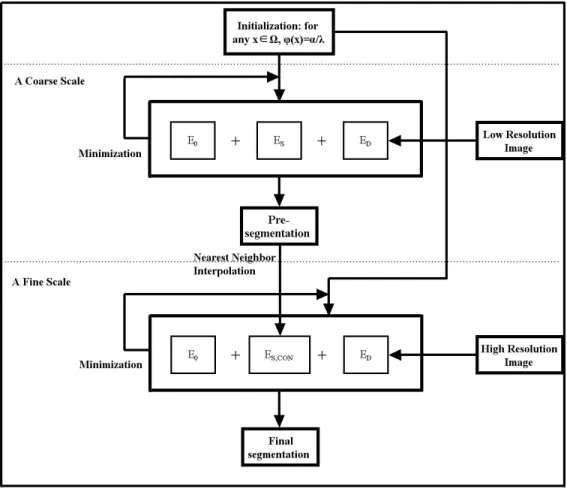
We have provided an efficient way to fix some of the parameters in terms of network width. In this chapter, we investigate the extraction of the highway network from a single QuickBird image. Since reducing the resolution eliminates high-frequency noise, the resulting pre-segmentation gives an approximate detection of the objects of interest.
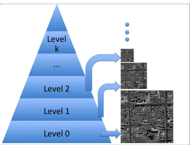
Multiresolution Analysis and Wavelets
The use of multiple resolutions thus allows the combination of coarse data – in which details in the image that could disturb the recognition process have been removed – with fine data for greater accuracy. Equation (3.3a) is called the wave equation, which relates the basic wave function to the scaling function at the next finer scale. The corresponding relation used in the inverse wavelet transform is s(j+1)l =X. 3.7) The direction from finer to coarser in equation (3.6) is called the process of decomposition or the process of analysis; the direction from coarser to finer in equation (3.7) is called the synthesis process of the reconstruction processor.
Model Definition at Multiple Resolutions
The resulting active contour is upsampled to a finer scale of the image and used as initialization. The process is continued on successively finer representations of the image until the active contour is developed in the image itself. On the other hand, thanks to the effects of other terms (mainly the data term), components of the object can still be extracted outside the pre-segmentation region.
Experimental Results and Comparisons
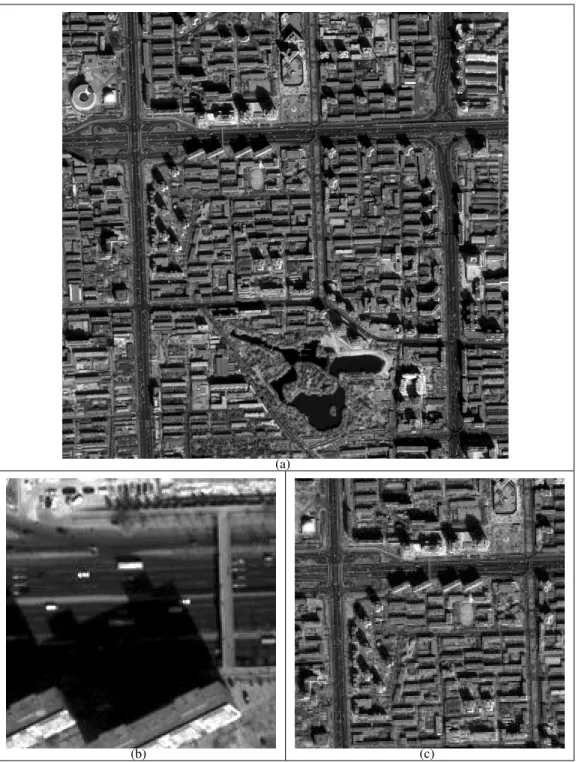
When we use the high-resolution EHR model instead, Figure 3.7(b) shows the final result on the original image. The experiments in Figure 3.6(a) at full resolution. a)-(b): results obtained with single-resolution primary energyEprimary and high-resolution EHR energy, respectively. If we still use the single-resolution Eprimary model, but on the full-resolution image, a large amount of false detections appear (see Figure 3.11(c)).
Conclusion
In the result at 1/4 resolution obtained with the primary model Eprimary (Figure 3.11(b)), the small road at the top right of the image is not included and the edges of the vertical main road are not very accurate. . Note that at full resolution the road in the top right corner is retrieved and also the position and width of the vertical main road are more accurate. For example, at the lowest end of the vertical road, the result in Figure 3.11(d) is closer to the actual image than that in Figure 3.11(b) due to the white road markings.
Introduction
Specifically, we show how to make use of an outdated digital GIS map and a recently acquired QuickBird image to generate a current road network of the observed region. Between the most general and the most specific is prior knowledge that comes from a common understanding of the object of interest. In the remainder of this chapter, based on the standard HOAC prior modelE0+ES, we introduce an additional specific prior termEGIS, derived from a legacy digital GIS map, to solve the above three aspects of road map updating.
Specific Prior Energy
In contrast, the most common prior knowledge concerns the regularity properties of the boundary∂Of the region of interestR. In this case of updating, the parameters of the Gaussian mixture and Gamma distributions in the data term are learned from the image data, using the known regionR0 to create examples of road and non-road. Note that the samples may contain errors, as R0 does not exactly match the road network in the image (e.g.
Experimental Results and Comparisons
The main effect is to eliminate false positives in the background, while maintaining the correct segmentation of the roads themselves. So in case the road network is extracted at full resolution while GIS data is not available, we can replace GIS information in the specific prior term with a low resolution result. We have already analyzed the disadvantages of the four methods we used in the previous chapter, but we will not repeat them here.
Conclusion
In previous chapters, we solved the problem of extracting and updating highway networks. Compared to the main roads, the secondary roads are much more difficult to deal with, because, on the one hand, of the low discriminative power of the gray level distributions of road regions and the background, and on the other hand, of the greater effect of closures and other noise on narrower roads . To tackle the above problems, in this chapter we show how to separate the control of branch straightness and branch width, thus enabling better extension of the network for a given path width.
Introduction
In other words, the length/range along which the network branch is expected to be straight is the same as the width of the branch itself. 1 To increase the size of the interaction function or to increase its range can be considered roughly equivalent. The first new energy term is the nonlinear, nonlocal HOAC ENL energy, which increases the magnitude of the interaction along one side of a network branch.

Nonlinear Nonlocal HOAC Prior Energy
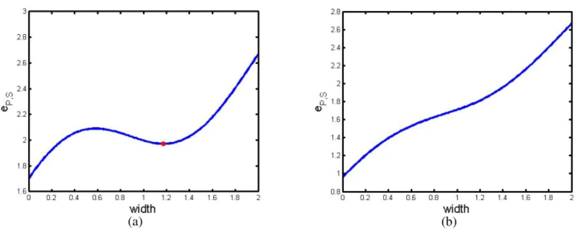
We decide to only adjust the size of the interaction (although this actually changes the size of the interaction as well). The above analysis shows that the stability of the nonlinear nonlocal joint HOAC prior model is related to the scaled control parameters ˆβ =β/α and ˆβ2 =β2/α and the scaled . We can now plot the relationship between the scaled control parameters βˆ and ˆβ2 and the scaled width ˆW.

Linear Nonlocal HOAC Prior Energy
On the other hand, when at least one of the two tangent vectors is nearly orthogonal to ∆γ, the product of the dot products is small. From the above it can be seen that γ(t0) exerts no force onγ(t), but for bothγL(t0) andγR(t0) the product of the dot products is negative. The energy has a very broad maximum (the inflection point of the three extremes) and a local minimum.
Experimental Results and Comparisons
The computational speed of the linear model is equal to that of the primal model;. In practice, the computation time of the linear model for this experiment is 60 minutes and 936 minutes at 1/4 and full resolution. To evaluate the performance of the new model, we now compare our result with other methods at full resolution.
Conclusion
To alleviate the problems arising from the complexity of the image scene at high resolution, we introduced a multiresolution statistical data model and a multiresolution constraint prior model. From the stability analysis of the linear non-local HOAC total prior model, we have shown that the model's behavior depends on the three scaled control parameters ˆβ, ˆβ2 and dˆ2. We can express the phase field preliminary model on a suitable wave basis, and develop the multiscale structure of the previous model.
Energy Terms of a Bar
In this appendix, we detail the calculation of the stability analysis of a long straight bar of length L and width W << L → ∞ (see Figure 2.5). Once this is done, we can introduce the variable η2=(z2+W2)/d2 for the second integral and again do not need the absolute value. Taking into account that ˆd2 = d2/d is the ratio between two interaction areas, we get the result in equation (5.24):.
Model Energy per Unit Length
Tolinear nonlocal HOAC total prior energy, per unit length of rod,eP,NL, is (see equation (5.13)). Since we decide to fix the value w in advance for the purpose of simplifying the problem, there is no need to calculate the second derivative with respect to tow. The linear non-local HOAC total previous energy, per unit length of rod, eP,L, is (see equation (5.26)).
Nonlinear Nonlocal HOAC Prior Energy
In this appendix we describe the calculation of the derivatives of the two new non-local HOAC preenergies proposed in chapter 5. F and F−1 denote the Fourier and the inverse Fourier transform, respectively, and a hat ˆ denotes the Fourier transform of a variable.
Linear Nonlocal HOAC Prior Energy
To avoid the calculation of convolution, we apply the Fourier transform to the above formula. In this appendix, we describe another term non-linear non-local HOAC prior ˜ENL, an alternative to ENL, which we do not use.
Because each term of ˜EHO includes a tangent vector, when changing from the contour formulation to the phase field formulation, it is not necessary to insert the boundary indicator function. Accordingly, the corresponding phase field energy is given by E˜HO(φ)=−1. C.4) The second term differs from ES. Obviously, ˜ENL is also a quarter in φ, but compared to ENL, this term leads to some implementation problems when performing the energy minimization.
After several intermediate steps, we find the first derivatives with respect to ˆW, and the second derivatives with respect to ˆW, of the above formulation. We see from these figures that, with the increase of ˆd2, the region where ˜eP,L has two local minima becomes larger; and in the energy plot the peak of the first local maximum becomes higher. Parameter setting is thereby facilitated, but a new problem arises: in this situation, we cannot control the amplitude of the first local maximum and the width of the flat minimum at the same time.

Method by Wang
In this appendix, we recall other methods in the literature that were used in this manuscript for comparison purposes.
Method by Yu
A set of candidate pixels whose gray values are in the road-specific spectral range [S1,S2] is extracted. For each candidate pixel, a set of straight segments with a predetermined length passing through this candidate pixel is obtained. Then, for each line segment, the ratio of the number of pixels whose gray value belongs to [S1,S2] to the number of all pixels in the line is checked.
Method by Bailloeul
Junction-aware extraction and regularization of urban road networks in high-resolution SAR imagery.IEEE Trans. Incorporating generic and specific prior knowledge into a multi-scale phase field model for road extraction from VHR image.IEEE Trans. Detection of linear features in SAR images: Application to road network extraction.IEEE Trans.