Optimal observability of the multi-dimensional wave and Schrödinger equations in quantum ergodic domains

We observe the restriction of solutions to a measurable subset Ω over a time interval [0, T] with T >0. We address the problem of optimal location of the observation subset ω among all possible subsets of a given mass or volume fraction.

Presentation of the problems

We refer to [42] for a thorough discussion of the problem of obtaining necessary and sufficient conditions ensuring the observability inequality, which is a wide open problem. When the spectrum is not simple, it is natural to consider an intrinsic variant of the second problem by considering the infimum over all possible normalized eigenfunctions (see Section 4.8).

Brief state of the art

Note that, when the spectrum of A is not simple, this spectral second problem depends a priori on the choice of the orthonormal basis (φj)j∈IN∗ of eigenfunctions. We also cite the article [55] where we study the related problem of finding the optimal location of the support of the control for the one-dimensional wave equation.

Short description of the main results of this article

Section 5 is devoted to the study of a finite-dimensional spectral approximation of the second problem, namely the problem of maximizing the functional. Of course, then, under the assumptions of the above theorem, these sets also form a maximizing sequence for the original optimization problem, without convexification.

Two motivations for studying the second problem

Note that, as is known, the assumption of simplicity of the Dirichlet-Laplacian spectrum is general with respect to the domain Ω (see e.g. The coefficients aj, bj and cj in the above expressions are the Fourier coefficients of the initial given, defined from (13) and (22) respectively.

Proofs of Theorem 1 and Corollary 1

However, note that, in this multi-dimensional case, this is due to the fact that the GCC may fail, but the minimal spectral trace overω is positive. The last equality is established by expanding the square of the sum within the integral, and by using the fact that the φk's are orthonormal in L2(Ω).

Proof of Theorem 2

There exists at least one measurable subset ω of Ω, solution of the first problem, characterized as follows. If ω were not symmetric with respect to this hyperplane, the uniqueness of the solution to the first problem would fail, which is a contradiction.

Further comments on the complexity of the optimal set

More specifically, it depends on their associated coefficients αij, defined by (16) in the case of the wave equation, and by (25) in the case of the Schr¨odinger equation. Its Fourier coefficients are the integer values ​​of the Fourier transform of the nonpositive triangle function, so they are negative and summed.

Several numerical simulations

Since J(a) is defined as the infimum of linear continuous functionals for the topology of the faint star L∞, it is semicontinuous above for this topology. Note, however, that although the Hausdorff topology has nice compactness properties, it cannot be used in our study due to the measure restriction on ω. We emphasize that the issue of the possible existence of a gap between the original problem and its convexified version is not obvious and cannot be addressed by conventional tools for Γ-convergence, in particular because the function J defined by (48) is not lower semi-continuous for the topology of the weak stars L∞ (but is semicontinuous from above for this topology as an infimum of linear functions).

This simple example illustrates the difficulty in understanding the limiting behavior of the functional due to the lack of the lower semicontinuity, which allows a gap to appear in the convexification procedure.

Main results

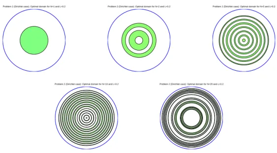
From this result, from Corollary 1 and Theorem 2, it follows that the maximum value of the randomized observability constants 2CT,rand(W) (χω) = CT,rand(S) (χω) over the setUL is equal to TL, and that if the spectrum of A is simple, the maximum value of the time-asymptotic observability constants is 2C∞(W)(χω) =C∞(S)(χω) over the setUL equal to L. We then set a similar (but different) result fixed within the class of measurable subsets whose boundary is measure zero. 53) This is the set of all characteristic functions of Jordan measurable subsets of Ω of measureLVg(Ω). Consider the Dirichlet-Laplacian on the domain Ωdefined as the unit disk of Euclidean two-dimensional space.

In order to establish this result, we use the explicit expression of certain semiclassical measures in the disk (weak limits of probability measures φ2jdVg) in the proof of this claim (done in Section 4.7).

Comments on ergodicity assumptions

Note that the fuzzy convergence of the measures µj is weaker than the convergence of the functions φ2j for the weak star topology of L∞(Ω). We refer to [9, 25] for results showing scarring on the periodic trajectories of the dynamics of the quantum Arnold's cat map. It is then proved in [68] that, on the standard sphere, almost every orthonormal basis of eigenfunctions of the Laplace satisfies the QE property.

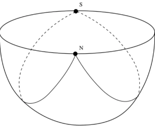
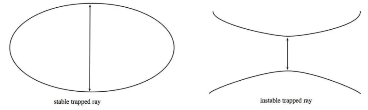
Their results showed that the quantum effects of bouncing balls or whispering galleries play an important role in the success or failure of the exponential decay properties.

On the existence of an optimal set

At the end of the article, the authors hypothesized that such considerations could be useful in the placement and design of actuators or sensors. For the two-dimensional square Ω = [0, π]2, which is studied in statement 2, we cannot give a complete answer to the question of existence. In fact, it easily follows from Lemma 5 and the proof of Proposition 2 that for L = 1/2 the supremum of J over UL is attained for every subset ω of the form.

In light of the results above, one would expect that when Ω is the unit N -dimensional hypercube, there exists a finite number of values ​​of L∈(0,1) such that the maximum in (52) is reached.

Proof of Theorem 4

Using once again similar arguments as in the proof of Lemma5 (Fourier transform and Plancherel's theorem), it follows that F must necessarily be continuous on [0, π]2 and thus constant. It is interesting to note that the optimal sets drawn on the left side of the figure do not satisfy the geometric control condition mentioned in Section 1.1 and that in this configuration the (classical, deterministic) observation constants CT(W)(χω) and CT(S )(χω) is equal to 0, whereas according to the previous results, Using the fact that the eigenfunctions are uniformly bounded in L∞(Ω), it is clear that f(x) ∈ ℓ∞, for every x ∈ Ω.

Proof of Theorem 5

First, we show that the set ωε still satisfies an inequality of the type (57) for sufficiently small Otherwise, we apply all previous arguments to this new set ω1: using QUE, there exists an integer still labeled j0 such that (57) holds with ω0 replaced by ω1. Finally, this leads to the existence of ω2 so that (67) holds, with ω1 replaced by ω2 and ω0 replaced by ω1.

Therefore, if the second problem is considered in the class of measurable subgroups ω of Ω, of measure Vg(ω) = LVg(Ω), which moreover are either open with a Lipschitz limit, or open with a perimeter of bounded, then the conclusion also holds that the supremum is equal to L.

Proof of Proposition 2

The lower frequencies j6j0 are then treated as before and we end up with (64) with ω0 replaced by ω1. By iteration, we construct a sequence of subsets ωk of Ω (which satisfy the δ-cone property) of measure Vg(ωk) =LVg(Ω) until J(ωk)< L, which satisfies. Since K is concave (as an infimum of linear functions), it suffices to prove that hDK(a=L), hi60 (the directional derivative), for every function h defined on Ω, such that R.

Applying the no-gap result in dimension one (obviously this can also be applied with the cosine functions), one has.

An intrinsic spectral variant of the second problem

The only thing to notice is the derivation of the estimate corresponding to (64). For every measurable subset ω of Ω, the sequence (JN(χω))N∈IN∗ is non-increasing and converges to J(χω). For any measurable subgroup ω of Ω, the sequence (JN(χω))N∈IN∗ is clearly non-increasing and thus convergent.

It follows from Sion's minimax theorem (see [61]) that there exists αN ∈ AN such that (aN, αN) is a saddle point of a bilinear functional.

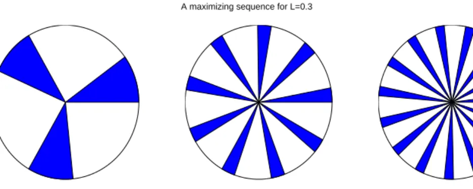
Numerical simulations: maximizing sequences

It is proved in [31, 54] that, in the one-dimensional case Ω = [0, π] with Dirichlet boundary conditions, the optimal set ωN maximizing JN is the union of N intervals centered around equidistant points and that ωN is actually the worst possible . subset for the problem of maximizing JN+1. In this section, we first consider in Section 6.1 classes of subsets that share compactness properties, with a view to ensuring existence results for the second problem (45) (uniform optimal design). In Section 6.2 we show how our results for the second problem can be extended to a natural variant of observability inequality for Neumann boundary conditions or in the unbounded case.

According to Lemma 5, we know that in the one-dimensional case the second problem (45) is ill-posed in the sense that it has no solution except L= 1/2.

Further remarks for Neumann boundary conditions or in the boundaryless case

Obviously, the optimal set then depends on the bound α under consideration, and numerical simulations (not reported here) show that, as α tends to +∞, the family of optimal sets behaves like the maximizing sequence constructed in Section 5, in particular the number of components of related increases with growth. Following the same lines as those in the proofs of Theorems 1 and 2 (see Sections 2.3 and 2.4), we obtain. First of all, it is easy to see that, in the definition of Γ, it suffices to consider the infimum over the real sequences (aj) and (bj).

Variant of observability inequalities and optimal design results

Let us first explain how to derive this expression in the case of the wave equation (the arguments are similar for the Schrödinger equation). This is due to the fact that on the left side of the observable inequalities (83) and (84) we use the H1 norm instead of the norm of D(A1/2). In the specific case in question (94) is replaced by the following statement: there exists N0∈IN∗ such that for ε >0 there exists L0∈(0,1) such that.

In the first three cases, the number of connected components of the optimal set seems to increase with N.

Optimal location of internal controllers for wave and Schr¨ odinger equations

According to the characterization of the optimal set in terms of a level set of the function. Proposition1 follows from that result, and the optimal set ω is then the complement of the fractal setC. Moreover, using the rationality of α, we can derive an estimate of below, as follows.

We have therefore constructed a function f that satisfies all requirements of the theorem, except the fact that f is smooth.