We note the restriction of solutions to a measurable subset of Ω in the time interval [0, T] with T >0. Considering the convexified formulation of the problem, we prove a gap-free result between the initial problem and its convexified version, under appropriate assumptions of quantum ergodicity on Ω, and compute the optimal value.
Problem formulation and overview of the main results
This leads us to rather consider an averaged version of the observability inequality over arbitrary initial data. Assume that there exists a subseries of the set of probability measures µj =φ2j(x)dx that converges vaguely to the uniform measure |Ω1|dx (weak quantum meridity assumption), and that the set of eigenfunctionsφj is uniformly bounded in L∞(Ω) .
Brief state of the art
This section is devoted to the discussion and mathematical modeling of the problem of maximizing the observability of the wave equations. A priori, it is natural to consider the problem of maximizing the observability constant CT(W)(χω) over all possible subsets ω Ω of the Lebesgue measure|ω|=L|Ω| for a given time T >0.
Spectral expansion of the solutions
In the sequel, the observability constant CT(W)(χω) denotes the largest possible non-negative constant for which inequality (12) holds, i.e. 13) We then discuss the issue of mathematical modeling of the idea of maximizing the observability of wave equations. Due to the crossed terms appearing in (17), the problem of maximizing CT(W)(χω) over all possible subsetsω of Ω of measure|ω|=L|Ω| very difficult to deal with, at least from a theoretical point of view.
Randomized observability inequality
The observability constant defined by (13) is defined as an infimum overall possible (deterministic) initial data. From this point of view, the deterministic observability constants are expected to be pessimistic with respect to their randomized version.
Conclusion: a relevant criterion
As we mentioned earlier, the problem of maximizing the deterministic (classical) observability constant CT(W)(χω), defined by (13) in all possible measurable subsets ω of Ω of measure|ω|=L|Ω|, is open and probably very difficult. For practical issues, it is actually more natural to consider the problem of maximizing therandomized observability constant defined by (24).
Time asymptotic observability inequality
If the domain Ω is such that every eigenvalue of the Dirichlet-Laplacian is simple, then. Section 3.1 is devoted to some preliminary remarks and especially to the introduction of a fluidized version of the problem (31).
Optimal value of the problem
From this result, from Corollary 1 and Theorem 4, it follows that the maximum value of the random observation constant CT,rand(W) (χω) over the set UL is equal to T L/2, and that, if the spectrum of △ is simple, the maximum value of the asymptotic observation constant of time C∞(W)(χω) over the setUL is equal to L/2. Then, for everyp∈(1,+∞] and for every basis of the eigenfunctions of △, the uniformLp-limiting property is not satisfied and QUE does not hold either.
Comments on quantum ergodicity assumptions
Second, they note that a stronger microlocal version of the QE property holds for pseudodifferential operators in the unitary cotangent bundle S∗Ω of Ω and not just in the configuration space Ω. Note, however, that here, as already mentioned, we are concerned with concentration results only in configuration space.
Proof of Theorem 6
We believe that if such an example exists, then the underlying geodesic current should be fully integrable and have strong concentration properties. As already mentioned in our framework, we have fixed a given basis (φj)j∈IN∗ for eigenvectors, and we only consider the weak limits for the measuresφ2jdx. We refer to Section 3.7 and especially to Proposition 2 for an example of a hole for an intrinsic variant of the second problem where the infimum runs over all possible eigenfunctions (and not just over a basis).
Their results reflected that the quantum effects of bouncing balls or whispering galleries play an important role in the success of failure of the exponential decay property. At the end of the article, the authors surmised that such considerations could be useful in the placement and design of actuators or sensors. In our opinion, this is the main contribution of our paper, in the sense that they pointed out the close connections between shape optimization and ergodicity, and provided new open problems and directions for domain optimization analysis.
Proof of Theorem 7
6 The isodiametric inequality says that, for every compactK of the Euclidean space IRn, |K|6 holds. First, let us show that setωε still satisfies a sufficiently small inequality of type (40). Otherwise, we apply all previous arguments to this new set ω1: using QUE, there exists a still-denoted integer j0 such that (40) holds with ω0 replaced by ω1.
The lower frequencies j6j0 are then handled as before, and we end up with (47) with ω0 replaced by ω1. Finally, this leads to the existence of ω2, so that (50) holds with ω1 replaced by ω2 and ω0 replaced by ω1. Therefore, if the second problem is considered on the class of measurable subsets ω of Ω, of measure |ω|=L|Ω|, which are furthermore either open with a Lipschitz boundary or open with a bounded perimeter, then the conclusion holds as well that the highest is equal to L.
Proof of Proposition 1
An intrinsic spectral variant of the problem
Assume that the uniform measure |Ω1|dxi is a closure point of the family of probability measures µφ =φ2dx, φ∈ E, for the fuzzy topology, and that the entire family of eigenfunctions inE is uniformly bounded in L∞(Ω). Assume that the uniform measure |Ω1|dx is the unique closure point of the family of probability measures µφ =φ2dx, φ ∈ E, for the fuzzy topology, and that the entire family of eigenfunctions inE is uniformly bounded inL2p(Ω), for someep∈(1,+∞]. The only thing to note is the derivation of the estimate corresponding to (47).
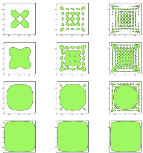
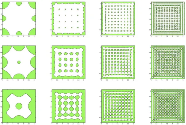
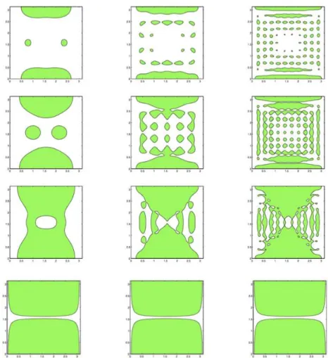
In Section 4.1 we investigate the question of the existence of an optimal set, reaching the highest point in (31). For the two-dimensional square Ω = (0, π)2 studied in Proposition1, we are unable to give a complete answer to the existence question. In light of the results above, one can expect that when Ω is the unit N-dimensional hypercube, there exist a finite number of values of L∈(0,1) such that the supremum in (37) is reached.
Spectral approximation
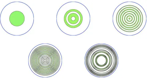
It is interesting to note that the optimal sets, drawn on the left side of the figure, do not satisfy the geometric control condition mentioned in section 2.1, and that in this configuration the (classical, deterministic) observability constants CT(W)(χω) and CT(S)(χω) are equal to 0, while according to the previous results 2CT,rand(W) (χω) = CT,rand(S) (χω) =T L holds. This fact is in agreement with Remarks 4 and 5. For any measurable subsetω of Ω, the sequence (JN(χω))N∈IN∗ is non-increasing and converges to J(χω). For any measurable subset ω of Ω, the series (JN(χω))N∈IN∗ is clearly non-increasing and thus convergent.
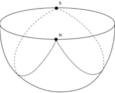
It follows from Sion's minimax theorem (see [55]) that there exists αN ∈ AN such that (aN, αN) is a saddle point of the bilinear functional. The eigenvalues of the Dirichlet-Laplacian are given by the dual sequence of −z2jk and are of multiplicity 1 if j = 0 and 2 if j > 1. Indeed, this is an immediate consequence of the uniqueness of a maximization for the modal approximation problem stated in Theorem 10 and that Ω itself is radially symmetric.
A first remedy: other classes of admissible domains
However, the point of view that we took in this paper is not to restrict the classes of possible subsetω, but rather to discuss the physical relevance of the criterion under study. In the next subsection, we rather consider a modification of the spectral criterion, based on physical observations.
A second remedy: weighted observability inequality
Under the assumptions of the theorem, there is no gap between the problem (64) and its convex formulation (65), as before. This result is due to the fact that we added the weight σ >0 to the left side of the observable inequalities. In the specific case in question (70) is replaced by the following statement: there exists N0∈IN∗ such that for ε >0 there exists L0∈(0,1) such that.
In the first three cases, the number of connected components of the optimal set seems to increase with N. Remedy: weighted observability inequalities In the general framework, the weighted versions (as discussed in Section 4.4) of the observability inequalities are (77) and (78). In Section 6.1 we show how our results for the second problem can be extended to a natural variant of observability inequality for Neumann boundary conditions or in the unbounded case.
Optimal shape and location of internal controllers
Along the same lines as in the proofs of Theorems 4 and 5, we obtain CT,rand(W) (χω) = T C∞(W)(χω) =TΓ,with. First of all, we can see that in the definition of Γ it is sufficient to consider the infimum over the real sequences (aj) and (bj). With this definition, it is a priori natural to model the problem of determining the best control domain as a problem of minimizing the norm of the operator Γω,.
Since Jω is convex, the first-order optimality conditions for the problem of minimizing Jω over L2(Ω,C)×H−1(Ω,C) are necessary and sufficient. We simply obtain the right-hand side, which states that the integral of a non-negative function over ω is lower than the integral of the same function over Ω, which allows the use of the orthogonal properties of φj. As already discussed in the paper, it is more relevant to maximize the randomized observation constant CT,rand(χω) defined by (24) (see Section 2.3).
Open problems
This question was investigated in [23] in the one-dimensional case, based on the two following remarks. Even a truncated version of this criterion is an open problem, that is, the problem of maximizing the lowest eigenvalue of the Gramian matrix whose element is rowj and columnkis R. In general, the question of the existence of an optimal set is completely open, and we expect that the supremum is not reached for generic domains Ω and generic values ofL.
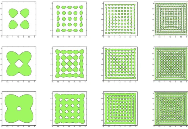
This conjecture is consistent with the observed increasing complexity of the sequence of optimal setωN solutions of the problem of maximizing the truncated spectral criterion JN. With the example of the disk (Proposition 1), we have seen that these assumptions are not sharp. Theorem11, which gives the existence of an optimal set for the weighted version of the problem, holds underL∞-QUE on the basis.