Dhiibbaa kaka’umsa lakkoofsa Strouhal qabbanaa’uu fiilmii irratti qabu” -iv- yeroo saffisi afuufuu battalaa saffisa afuufuu giddugaleessaa gadi ta’etti dallaadhaaf barbaachisaa dha. Dhiibbaa kaka’umsi lakkoofsa Strouhal qabbanaa’uu fiilmii irratti qabu” -ix- 4.4.33 Teempireecharri ddessccrriippttiioonn ooff tthhee wiwinndd ttuunnnneell flflooww ChChaarraacctteerriizzaattiioonn ooff iinnjjeeeccttaanntt.1 f1flloowww21nntt.
INTRODUCTION
- Scientific and industrial context
- Techniques for material protection
- Materials
- Thermal barrier coating
- Cooling with air injection
- Flow field unsteadiness of gas turbine engine
- Organization of the manuscript
- References
Influence of Strouhal number excitation on film cooling" -9- the thesis is divided into chapters 2 to 8, which comprise the chapter of bibliography, experimental set-up and measurement techniques, characterization of upstream flows, study of the film-cooled boundary layer flow aerodynamics, study of the wall heat transfer in film cooled boundary layer (infrared thermography), study of the film cooled boundary layer flow temperature (cold wire measurements) and conclusion. Finally, the recent developments on the issue of the jet pulsation affecting film cooling effectiveness are summarized.
BIBLIOGRAPHICAL REVIEW
Definition of Jet-in-crossflow
Some of these include the take-off and landing of the VTOL aircraft (vertical take-off and landing), film cooling of gas turbine systems, mixing the pollutant with the crosswind, mixing two different power streams in a combustion chamber. The resulting flow field for these configurations is usually quite complex and the flow field characteristics depend significantly on the velocity ratio (R=Ui U∞), the density ratio (D.R=ρi ρ∞) and the Reynolds number of both mainstream (Re∞ = U .∞ d ν ) and injection (Rei =Ui.d ν ) currents (where; d=hole diameter).
Description of the aerodynamics of a jet in crossflow
- Flow field at low Reynolds number flow
- Flow field at high Reynolds number flow
- Development of the flow field in the wake region
- Shedding frequency of wake structures
- Influence of a slightly heated jet on the JICF
They both concluded that the vortex structures in the wake are formed by the vortex originating from the boundary layer of the crossflow wall. The study of the vortex structures in the wake of a transverse jet emitted in a crossflow was carried out by Fric and Roshko (1994).

Description of aerodynamic and heat transfer of an inclined Jet in crossflow applied to film cooling
- Aerodynamic description
- Thermal description
- Fundamental parameters of film cooling analysis
At the inclined beam, the strength of the vortex systems is relatively low. The strength of the flow vortex is much higher in the case of a normal jet (the part of the jet stream near the tube exit was not shown for a normal jet).
UMi U
Geometrical parameters
Influence of Strouhal number excitation on film cooling” -27- ratio of parameters as follows; coolant-to-mainstream density ratio (D.R.), velocity ratio (R.), mass flux ratio (M), and momentum flux ratio (I). Influence of Strouhal Number Excitation on Film Cooling” -29- At larger angles, the flow tends to rise from the surface and wall protection is significantly reduced.
Influence of aerodynamic parameters on wall heat transfer
They suggested that the reduced levels of ηc for lower density ratios can be attributed to the lower blowing ratio at the same momentum flux ratio. 1996) have investigated the film cooling efficiency for various hole geometries as a function of the momentum flux ratio 'I'. Influence of Strouhal Number Excitation on Film Cooling" -34- holes 'P' and length to diameter ratio 'L/d' were 3d and 4 respectively.
Application of periodic velocity boundary limit on flow structure and wall heat transfer
- Flow from a submerged pulsating jet
- Effect of turbine flow unsteadiness on film cooling
- Characterization of turbine unsteadiness through bulk flow pulsation
- Characterization of turbine unsteadiness through injectant flow pulsation In these studies, the pulsation frequencies are chosen to maintain a condition of injectant
- Influence of jet Strouhal number pulsation on film cooling effectiveness Coulthard et al. (2006a) experimentally investigated the effects of jet pulsation on a flat
They reported that at low frequency pulses (St= f *d/U∞<0.8), the film cooling provided performance comparable to the time-weighted average performance of the steady beam. However, they mentioned that the dynamics of the jet at higher frequency are quite complex.

Conclusion
Influence of Strouhal number excitation on film cooling” -48- experimental and computational aerodynamics of internal flow, July Prague. 51 Yuen CHN, Martinez-Botas RF, “Film cooling characteristics of a single circular hole under different flow angles in a cross-flow: Part I, Effectiveness”, Int. 53 Yuen CHN, Martinez-Botas RF, "Film cooling characteristics of rows of circular holes at different flow angles in a cross-flow: Part I, Effectiveness", Int.
Frame work of experimental measurement
A common practice used in film cooling experiments is to use the hot fluid jet in the wall injection and the cold fluid jet in the mainstream (i.e. changing the inlet thermal state of the interacting flows). This means that the influence of the invigorating effect is very small in the current conditions. A simple scaling model used to simulate the film cooling problem in the present study involves an ordinary flow and a 30° inclined injector flow interacting over a flat wall, see figure (3.2).
Principle hardware components
- Wind tunnel
- Test section
- Injection plate
- Injection Flow System
- Measurement of injection mass flow rate
- Heating system for injectant flow
- Injectant temperature regulation system
- Pulse generation system
Table-3.1 : Description of the insulating materials used at the bottom of the injection plate. The flow rate in the supply branch of the injection flow is maintained by an orifice tube. The second part of the enclosure covers the lower part of the speaker and represents the lower side volume.
Velocity measurement systems
- Laser Doppler Anemometry
- Descriptions of the measurement scenario
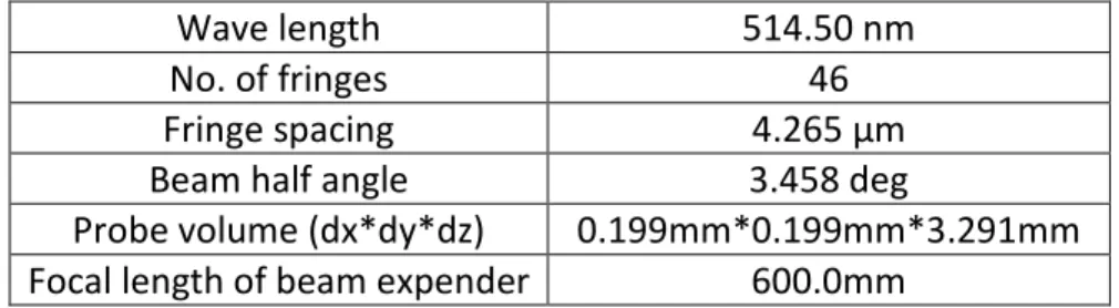
- Experimental conditions for LDV measurements
- Working principle
- Hot wire Anemometer
- Descriptions of the measurement scenario
- Experimental conditions for hot wire measurements
- Working principle
- Statistical errors in LDV and hot wire measurements
- Time Resolved Particle Image Velocimetry
- Descriptions of the measurement scenario
- Experimental conditions for TR-PIV measurements
- Fundamentals of PIV system
- Spatial resolution of PIV system
- Statistical errors in TR-PIV measurements
Since then, the hot wire measurements have actually been carried out in the initial phase of the thesis. Influence of Strouhal Number Excitation on Film Cooling” -70- with LDV, as one of the Reynolds numbers in hot wire testing is almost twice as high as the highest Reynolds number studied with LDV. In the later situation they kept the temperature of the air in the injection plenum at 150 K.
Thermal measurements of film cooling configuration
- Infra-red thermography
- Descriptions of the measurement scenario
- Experimental conditions for TR-PIV measurements
- Injection wall heat dissipation system
- Infra-red camera
- Surface temperature map (without flow)
- Cold wire measurement
- Descriptions of the measurement scenario
- Experimental conditions for cold wire measurements
- Working principle
A schematic diagram showing the basic arrangements used for infrared thermography of the injection wall is shown in figure (3.24). The emissivity of the present test wall (painted black) was measured by Dieumegard (2003) under identical arrangements to be (ε. In the cold wire experiments the temperature ratios of the interacting flows were maintained at Ti T∞=40/40= 2.

Data treatments
- Phase average description of the flow
- Turbulence description of the flow
- Convective heat transfer coefficient and adiabatic wall temperature
- Heat transfer Models
- Steady state heat transfer model
- Convective heat flux
- Phase averaged description of the temperature field
- Thermal uncertainties
The flat part of the curve corresponds to existing degrees in the inertial zone with uniform mean degrees of dispersion. In this model, hcf was represented by a thermal exchange in the iso-energetic state, (T∞=Ti). The subscript cf stands for cold flow because the temperatures chosen were close to ambient temperature. The model consists of determining the wall temperature distribution at different convective heat fluxes and using linear heat exchange characteristics to specify both the convective heat transfer coefficient and the adiabatic wall temperature.

Petre B, Dorignac E, Vullierme JJ, "Investigation of the influence of the number of hole rows on the convective heat transfer in the case of full-coverage film cooling", Int. Saumweber C, Schulz A, "Interaction of film cooling rows: effects of hole geometry and row spacing on the cooling performance downstream of the second row of holes", ASME Journal of Turbomachinery. Teekaram AJH, Forth CJP, Jones TV, "The use of foreign gas to simulate the effects of density ratios in film cooling", ASME Journal of Turbomachinery.
CHARACTERIZATION OF UPSTREAM FLOWS
Velocity characterization of wind tunnel flow
- Evolution of mean and rms velocities
- Viscous scales
- Comparison of velocity profiles
- Turbulence intensity
This scale is used in the following sections to represent some of the turbulence parameters. Therefore, we can locate some profile points in the viscous sublayer. The friction velocity is calculated using the logarithmic law, since there are many points available in the logarithmic range.

Description of turbulence scales and energy spectra
- Energy spectrum
- Turbulence length scale
The profiles of the integral length scale are shown in figure (4.10), which illustrates an increase in the integral length scale with respect to the Reynolds number of the flow. So it becomes difficult to determine the inertial length scale in the central region of the test section by the graphical method. The results depict a small gradual increase in scale size towards the edge of the boundary layer for all profiles.
Temperature description of the wind tunnel flow
Effect of Strouhal Number Excitation on Film Cooling” -120- It was found that the system reaches a uniform temperature in the main stream after one and a half hours when the control temperature of the stream in the wind tunnel is set to 20 °C. Flow temperature measurements in the wind tunnel were performed to determine the uniformity of the temperature field developing along the test section of the wind tunnel. The mean velocity of the wind tunnel was set at 10 m.s-1 (Re=8609), while the flow control temperature was maintained at 20 °C.
Characterization of injectant flow
- Velocity profiles at the hole exit
- Characterization of pulsation amplitude
These measurements enable us to adjust the pressure regulator located on the upstream side of the injection flow distribution system for the required nominal flow rate at the hole exit. Average phase velocity values at different time instants are estimated by performing integral averaging of the velocity profile derived from the phase-locked results at the hole exit. The maximum deviation of the increase of the signal amplitude for the extreme cases of pulsation (M =0.65, St=0.2; M =1 and 1.25, St=0.5) as the fluctuating components of the speed are filtered.
Energy spectra
Influence of Strouhal number excitation on film cooling” -126- is approximately St=0.16 near a velocity ratio of 2. Levi (1983) reported the law of Strouhal number for the periodic phenomena occurring in different flows; including wakes behind cylinders, fluttering turbulent aircraft jets, flow over cavities and Von Karman eddies, etc. They suggested that the St is on the order of 0.159, despite little to no similarity between these flows.
Comparisons of baseline results
The small shift in these profiles is due to higher injection angle and injection Reynolds number (Rei), 35° and 15000, in the reference case and 30° and 8437 in this study. Higher injection Reynolds number in the reference case for M = 1 causes a small increase in streamwise mean velocity profile compared to the profile obtained from the present case. The injection angle of the jet fluid is identical for both studies, but a slightly thicker boundary layer flow in the reference case allows a deeper penetration of the jet into the mainstream flow compared to the present study.
Conclusion
This is due to the diversion of jet fluid downstream by the main flow. The energy spectra determined from the wake region of the flow have shown an almost constant Strouhal number St∞=0.15. The comparison of the basic results shows that the test setup is well calibrated, as the current results appear to approximate the previously reported results with reasonable deviations.
Yuen CHN, Martinez-Botas RF, "Film cooling characteristics of a single round hole at different angles to the flow direction in a cross flow: Part I, Effectiveness", Int.
STUDY OF THE FILM-COOLED BOUNDARY LAYER FLOW AERODYNAMICS
Structure involved in the flow dynamics
The size of the wake area can vary due to the small unsteady variations in the dynamics of the upstream currents. The vertical structure emerging from the tube consists of the vortex that arises in the boundary layer of the injection tube. The interaction creates a strong shear layer in the region of the interface of two flows.
Velocity field
- Time-averaged velocity
- Phase-averaged velocity results
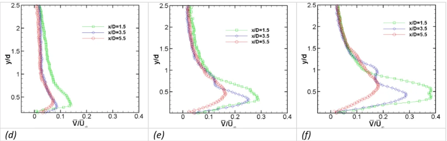
Figure (5.6d-f) shows the profile of the time-averaged wall normal component of the velocity for the cases of M = 0.65, 1 and 1.25, respectively. Such variation reduces the time-averaged velocity gradient in the shear region of the flow field for M = 0.65. Influence of the Strouhal number excitation on the cooling of the film” -141- to detach from the wall and a relatively stronger bound vortex forms, allowing greater secondary movement of the main stream under the jet.
Velocity probability density function (PDF)
Influence of Excitation of Strouhal Numbers on Film Cooling” -146- At M =1.25, the PDF for both u and v shows a slight negative skew in all cases of St, with the skewness for u being close to zero and -0.3 for v at St= 0.3. The pulsation at St=0.2 and 0.3 seems to increase the flatness factor slightly compared to the cases of St=0 and St=0.5 for v. For M =1.25 the flatness of the PDF increases for v at St=0.2 and 0.3 in the same way as for the other bladder ratios, while the skewness becomes positive for both u and v.

Turbulent description, tensor of Reynolds stresses
- Time-averaged normal stresses
- Time-averaged shear stresses
- Phase-averaged shear stresses
- Ratio of phase-averaged rms-velocity components
- Phase-averaged turbulent intensity
In the case of M =1.25, the profile becomes slightly more uniform along the expected jet boundary. Some significant turbulence produced in the upper region is probably due to the interaction of the mainstream and the systematically collapsing jet fluid. However, the observed jet fluid turbulent intensity is about 7% in the core potential region lying close to the jet exit.

Tensor of velocity gradient
- Time-averaged vorticity
- Phase-averaged vorticity
- Time-averaged rate of deformation
In the downstream flow, the maximum positive peak of each profile always remains at the lower boundary of the jet. This results in a certain pattern of spray distribution and the deformation rate in the wake of the flow field and the lower boundary of the jet. At higher blowing ratios of M = 1 and 1.25, the deformation rate is more developed in the boundary region of the jet.
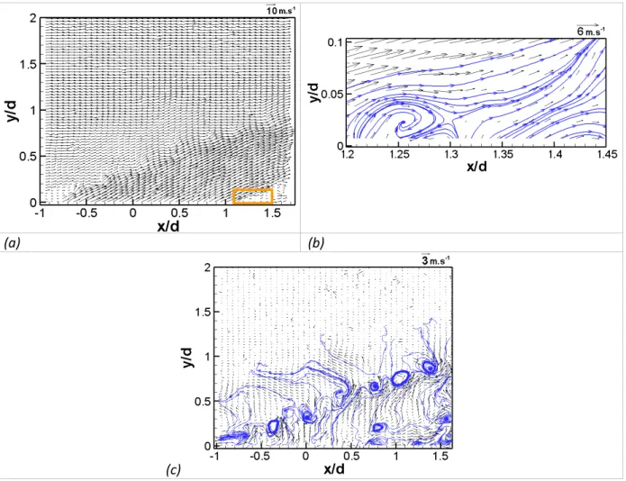
Vortex identification
Therefore, we can think that the sign of rotation of the vortex lying in the wake region is correct. Pulsation appears to cause the mixing of the flow, which relates to the wake region and the jet. At M =1.25 and St=0.5, as shown in figure (5.29g-i), the resulting flow field shows more frequent splitting of the jet and short span variations in the wall-normal direction as M =1 and St=0.5.
Mass, momentum and energy conservation
- Balance of mass (Continuity equation)
- Balance of momentum
- Terms of momentum equation, time-averaged results
- Balance of energy
- Terms of Energy equation, time-averaged results
- Time-averaged turbulent kinetic energy
The peaks in the Reynolds stress gradient profiles lie slightly below this region. The unknown cross-stream effective velocity (w2) is determined using the approximation w2=(u2+v2)/2. For the profiles shown in figure (5.34), the contribution of P*k,nor to the total production in the peak area is 62%.


