Cette thèse porte sur le problème de la reconnaissance de l'action, c'est-à-dire la détermination du type d'action en cours, ainsi que de sa localisation temporelle. Nos approximations conduisent à des accélérations d'au moins un ordre de grandeur tout en conservant des performances de pointe en matière de reconnaissance et de localisation d'actions.
List of Tables
Introduction
Contents
- Context
- CONTEXT 3 researchers directed their efforts on the problem of action recognition and
- Goals
- GOALS 5
- Contributions
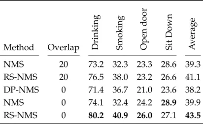
- CONTRIBUTIONS 7 propose a variant of NMS that corrects this issue without introduc-
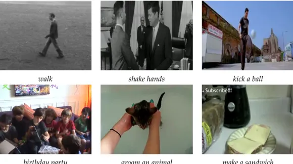
Action Recognition The goal of recognition is to assign a query video to one of the given classes. The task of the challenge is to evaluate the action recognition and localization approaches in real conditions.

Related work
- Action recognition
- Local features
- ACTION RECOGNITION 11 as, motion segmentation and tracking, and, as a consequence, they have
- Encoding methods
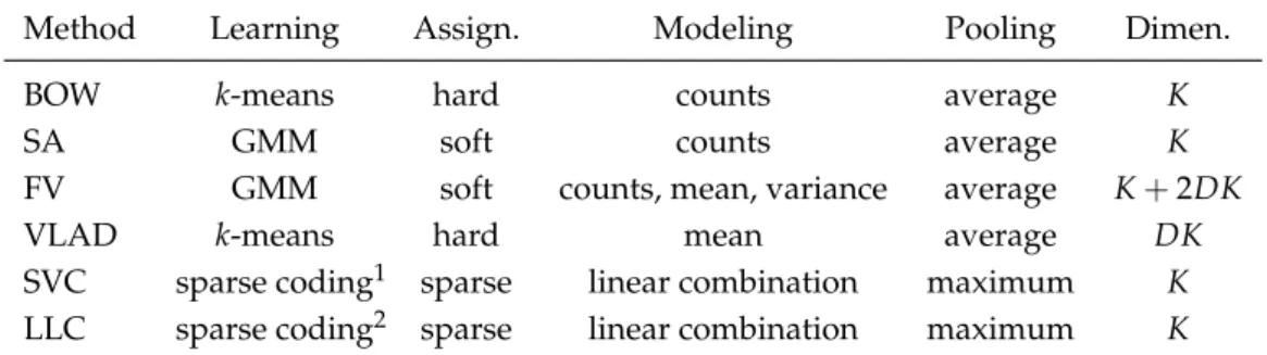
- ACTION RECOGNITION 13 We distinguish three stages for a quantization-based encoding tech-
- ACTION RECOGNITION 15 on the unit sphere, trying to avoid the problem of meaningless distances
- Deep learning
- Event recognition
- Complementary features
- EVENT RECOGNITION 19 techniques into three types, according to the place where we fuse the
- High-level features
- EVENT RECOGNITION 21 the type, the specificity and the quality of the detectors in the context
- Structured models
- Localization
- LOCALIZATION 23 localization and in Subsection 2 we review ways of dealing with the
- Models for localization
- Efficiency
- LOCALIZATION 25 sum of window scores)
Gaidon et al.[2013] use efficient image compositing techniques to calculate the approximate motion of the background plane and generate stabilized videos before extracting dense trajectories [Wang and Schmid, 2013] for activity recognition. Wang et al.[2012b] investigate the coding methods together with different pooling approaches (maximum and average) and normalizations (`1and`2).
A robust and efficient video representation for action
- Local features
- LOCAL FEATURES 29
- Dense trajectory features
- Improved trajectory features
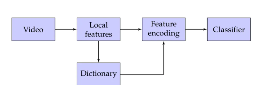
- Feature encoding
- Bag of words
- FEATURE ENCODING 33
- Fisher vector
- FEATURE ENCODING 35
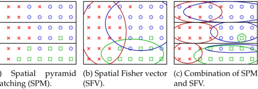
- Weak spatio-temporal location information
- Classification
- Non-maximum-suppression for localization
- NON-MAXIMUM-SUPPRESSION FOR LOCALIZATION 39
- DATASETS USED FOR EXPERIMENTAL EVALUATION 41
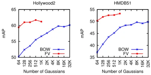
A common normalization technique is to divide the histogram scores by the number of features; this ensures that the representation is invariant with the size of the video. a) The bag of words (BOW) encoding. As we will see later in the experimental part (Section 3.6.1), the BOW representation can achieve comparable performance to FV, but at the expense of working with very large codebooks (several orders of magnitude larger than FV).
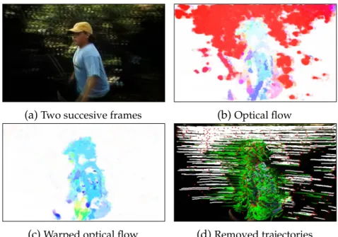
![Figure 3.1 – The steps of computing dense trajectories [Wang et al., 2013a].](https://thumb-eu.123doks.com/thumbv2/1bibliocom/464765.70213/44.892.130.696.197.379/figure-steps-computing-dense-trajectories-wang-et-2013a.webp)
- Datasets used for experimental evaluation
- Action recognition
- DATASETS USED FOR EXPERIMENTAL EVALUATION 43 sequences for testing as recommended by the authors. We report mAP
- Action localization
- Event recognition
- Experimental results
- Action recognition
- EXPERIMENTAL RESULTS 47
- EXPERIMENTAL RESULTS 49
- EXPERIMENTAL RESULTS 51
- EXPERIMENTAL RESULTS 53 [2013] report 83.3% using randomly sampled HOG, HOF, HOG3D and
- Action localization
- EXPERIMENTAL RESULTS 55
- Event recognition
- EXPERIMENTAL RESULTS 57 does not improve the results. This happens because the events do not
- EXPERIMENTAL RESULTS 59
- Conclusion
As features we use HOG+HOF+MBH of enhanced trajectory features but without human detection. We see a dramatic improvement when comparing our result of 31.6% to the state of the art.
Efficient localization with
Related work
RELATED WORK 63
The recent work of Li et al [2013b] is an exception to this trend; omitted PV power normalization, but presented an efficient approach to include accurate '2normalization. In this way, a set of only 1000 to 2000 windows is sufficient to capture 95% of the objects in the PASCAL VOC datasets.
Approximate Fisher vector normalization
- The Fisher vector and its normalizations
APPROXIMATELY NORMALIZED VISSER VECTORS Most of the recent work using FV representations for object and action localization, and semantic segmentation, either use non-normalized FVs [Chen et al., 2013, Csurka and Perronnin, 2011], or explicitly compute normalized FVs for all considered windows as in [Cinbis et al.,2013] or as in Chapter3. This representation has a size only three times larger than a local BOW histogram, while leveraging the representational power of the normalized FV.
- Approximate power normalization
APPROXIMATELY NORMALIZED FISHING SERVICES Other interpretations of the power normalization are given in [Winn et al.,2005,Perronnin et al.,2010,J´egou et al.,2012,Cinbis et al.,2012]. Cinbis et al.[2012] have argued that the power normalization corrects for the independence assumption made in the GMM model underlying the FV representation.
APPROXIMATE FISHER VECTOR NORMALIZATION 67 Based on this analysis, we propose an approximate version of the
- Approximate ` 2 normalization
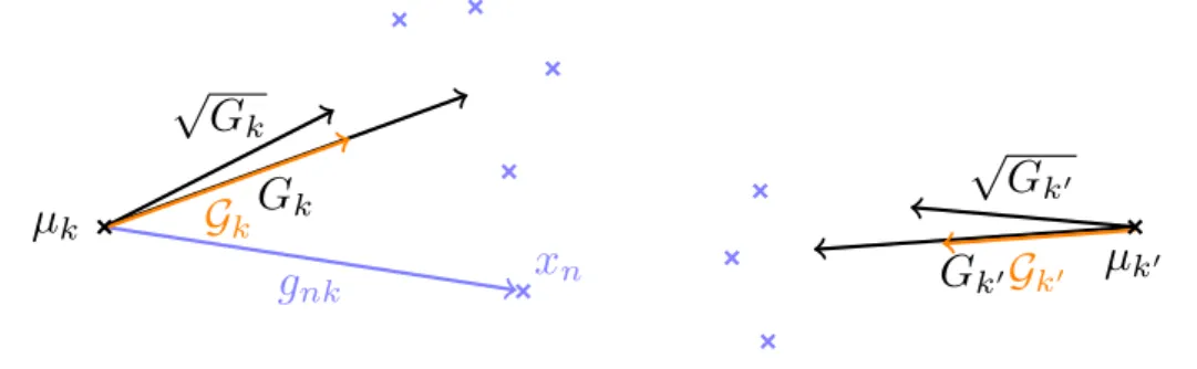
APPROXIMATE FISHER VECTOR NORMALIZATION 67Based on this analysis, we propose an approximate version of . Our approximate normalization Gk scales the magnitude of the Fisher vector Gk in contrast to the exact power normalization√.
APPROXIMATE FISHER VECTOR NORMALIZATION 69
- Complexity of approximately normalized FVs
Now we use the following two assumptions to cancel the second term from the right-hand side and complete the proof: (a) the data are i.i.d., so the expected value is multiplicative, i.e. E[XY] =E[X]E [Y]for X,Y i.i.d. We combine the above approximations to calculate a linear function of our approximately normalized FV as. 4.12).
APPROXIMATE FISHER VECTOR NORMALIZATION 71 Combining these formulations we obtain the classification score as a ratio
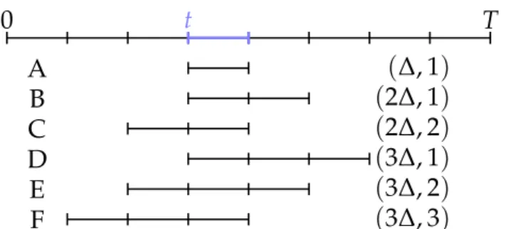
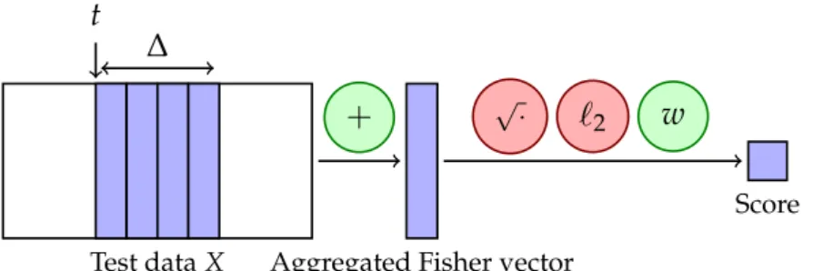
First, we precalculate the scores for each individual temporal slice by calculating the dot product X>wof the data matrix X with the classification weight. In each case, we obtain the data matrix X ∈ R2Kd×C, which contains a Fisher vector for each temporal slice, and the goal is to score a given time interval starting at slice and lasting for ∆slices.
APPROXIMATE FISHER VECTOR NORMALIZATION 73
The initial set of possible windows contains all the windows that start between slow and high and end between low and high (parent). The boundary step, which we illustrate for the parent, depends on quantities calculated at the intersection (A∩) and union (A∪) of all windows.
Integration with branch-and-bound search
INTEGRATION WITH BRANCH-AND-BOUND SEARCH 75
- Upper-bound for additive linear classifiers
We obtain the top quindows by running the branch-and-bound algorithm ktimes, removing the selected window from the search space after each iteration. INTEGRATION WITH BRANCH-AND-BOUND SEARCH In particular, consider such a function over the non-normalized FVG:.
INTEGRATION WITH BRANCH-AND-BOUND SEARCH 77 particular, consider such a function over the non-normalized FV G
- Bounding approximate power-normalization
- Bounding with approximate ` 2 norm included
If the intersection A∩ is nonempty, we can bound the second term by summing over the intersection, and obtain the lower bound onL(G) as: . 4.22) If the intersection is empty, instead of the sum overA∩, we can use the minimum overA∪ to obtain the boundary:.
Experiments
APPROXIMATELY NORMALIZED FISHER VECTORS Then it is easy to see that the result can be upper bounded as . 4.20) Since the latter limit relies on the non-linear max operation, it cannot be efficiently calculated using integral images.
EXPERIMENTS 79 evaluation protocol can be found in the previous chapter, see Section 3.5
- Effect of approximation on action classification
This standardization can be absorbed in the classifier weight vector w before the local scoren is calculated, and therefore does not affect the computational efficiency of our approach.
EXPERIMENTS 81
- Temporal action localization
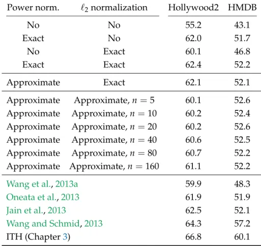
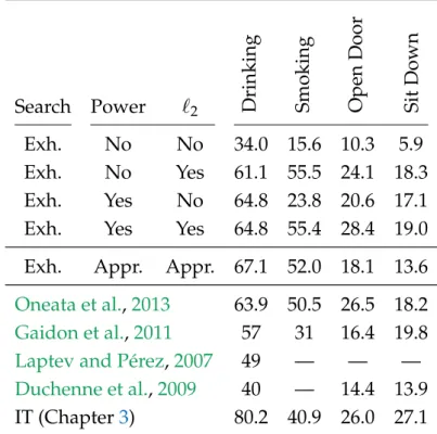
As before, the first four results consider the impact of exact normalizations on performance. Binge drinking and reducing power and normalizing `2 have a similar impact and improve scores by about 30 and 12 mAP points, respectively.
EXPERIMENTS 83
Although faster than exhaustive search, the speed obtained using branch-and-bound is generally limited. We expect greater speedup for branch-and-bound when applied to 2D spatial or 3D spatio-temporal localization problems.
Conclusion
Both exhaustive and branch-and-bound searches first preprocess all the cells in the temporal grid to compute the local sums of scores, assignments, and norms. When only the vertex window is required, branch-and-bound search can further speed up localization by a factor between 2 and 4, excluding preprocessing.
Spatio-temporal proposals
Related work
- Supervoxel methods
- Object proposals for detection in video
Unlike Xu et al [2013], however, we do not limit ourselves to finding a single video segmentation, but instead allow for overlap between different detection hypotheses. Yuan et al [2009] proposed an efficient branch-and-bound search method for locating actions in spatio-temporal frames, based on efficient sub-window search [Lampert et al., 2009a].
RELATED WORK 91 that is more general and applies to arbitrary representations is the use of
2015] starts with object proposals for each frame, ranks them using a moving objectivity score and then temporally expands the most promising ones based on dense optical flow. In our experiments, we compare with the results of Papazoglou and Ferrari[2013] on the YouTube Objects dataset.
Hierarchical supervoxels by spatio-temporal merging
- Construction of the superpixel graph
They refine the window-based solution using a pixel-wise MRF. Papazoglou and Ferrari [2013] proposed a method that uses motion boundaries to estimate the perimeter of the target object, and refine these estimates using an object appearance model.
HIERARCHICAL SPATIO-TEMPORAL SEGMENTATION 93
- Hierarchical clustering
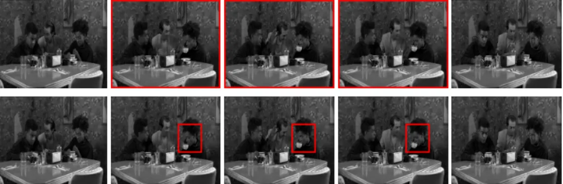
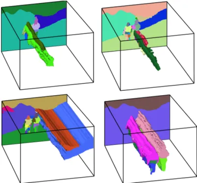
Because the graph is sparse, the clustering can be computed efficiently: if the number of connections per superpixel is independent of the number of superpixels – as is the case in practice – the complexity is linear in the number of superpixels. While such a clustering approach gives good results for image segmentation [Arbel´aez et al., 2011], its temporal extension tends to group clusters corresponding to different physical objects that are only accidentally connected in a small number of frames, see Figure 5.3.
HIERARCHICAL SPATIO-TEMPORAL SEGMENTATION 95
Spatio-temporal object detection proposals
- Randomized supervoxel agglomeration
SPATIO-TEMPORAL OBJECT DETECTION PROPOSALS 97
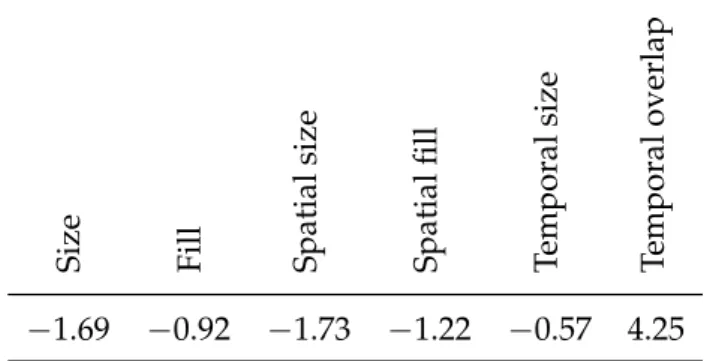
- Learning supervoxel similarities
The volumes an and am are normalized by dividing by the volume of the complete video. The fill feature that favors merging of supervoxels forming a compact region, and measures the extent to which the two supervoxels fill their bounding box: ffill(n,m) = (an+am)/bnm, where bnm is the volume of the 3D bounding box of the two supervoxels, again normalized by the video volume.
Experimental evaluation results
- Experimental setup
The 3D sub-segmentation error averages the following error over all ground truth segments: the total volume of intersecting supervoxels minus the volume of g, divided by the volume of g. Similar to the evaluation of 2D object proposals in [Uijlings et al., 2013], we measure performance using the best average overlap (BAO) of proposals with ground truth actions and objects.
EXPERIMENTAL EVALUATION RESULTS 101 annotated frames. More formally
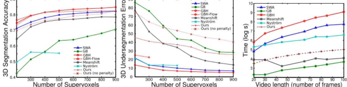
- Experimental evaluation of supervoxel segmentation
In terms of segmentation accuracy (left), our method is comparable to the best methods: GBH and GBH-Flow. The discrepancy in evaluation results across these measures is due to the fact that our method tends to produce larger supervoxels as well as many tiny supervoxels consisting of single isolated superpixels.
EXPERIMENTAL EVALUATION RESULTS 103
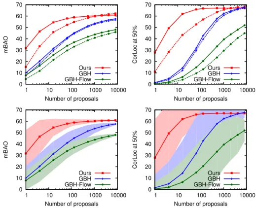
- Evaluation of spatio-tempoal detection proposals
In the lower plots, the filled area indicates the standard deviation of the performance given multiple examples of proposals. The full-time time limit, which accepts suggestions only if they span the full duration of the video, improves results for all methods.
EXPERIMENTAL EVALUATION RESULTS 105
We vary the number of suggestions by changing the level of the segmentation: we start with the suggestions generated from the coarsest segmentation and incrementally add suggestions obtained at finer levels. Figure 5.12 shows the results for DP and the random fusion algorithm, random Prim (RP), for the three segmentation methods.
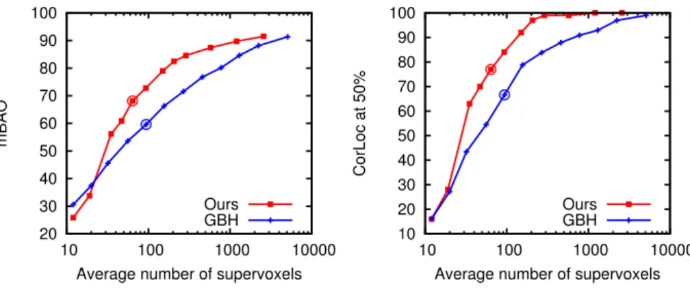
EXPERIMENTAL EVALUATION RESULTS 107 segmentations, RP outperforms DP as we generate more proposals. On
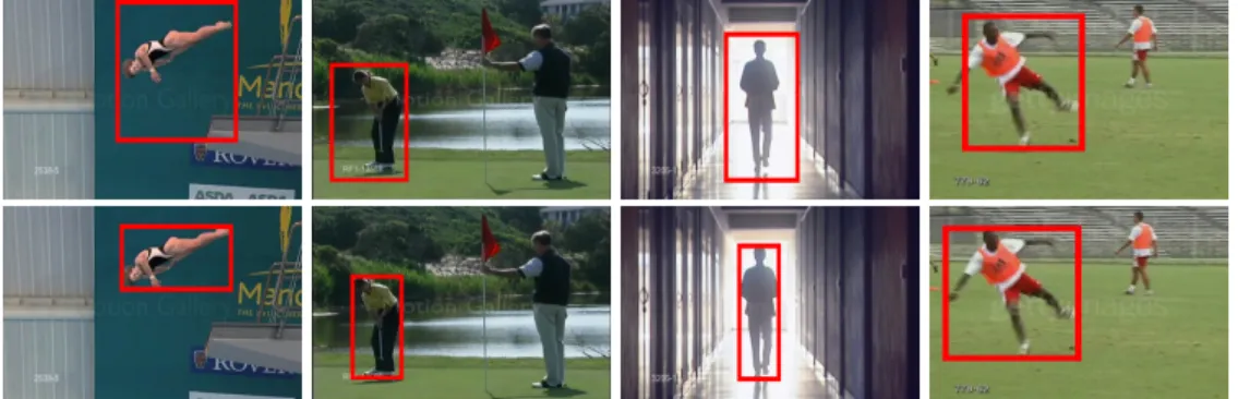
The video object segmentation approach of Papazoglou and Ferrari [2013] is unsupervised and produces only a single segmentation per recording. Compared to the video object segmentation method of Papazoglou and Ferrari [2013], our method achieves similar results when using 16 proposals, but we further improve when more proposals are used. Perst et al. [2012a] obtain similar results to ours with a single proposal. proposal, but their method is class dependent.
EXPERIMENTAL EVALUATION RESULTS 109
- Discussion
Conclusion
Conclusions
- Summary of contributions
- FUTURE RESEARCH PERSPECTIVES 113
- Future research perspectives
These hierarchical approaches achieve variety by either changing the base segmentations [Van de Sande et al.,2011] or the. Similar to [Manen et al.,2013], our method uses supervision to learn a weight combination for the different features.
Publications
International conferences
Journal submissions
Other publications
Bibliography
Bag of visual words and fusion methods for action recognition: Comprehensive study and good practice. Action recognition in videos captured by a moving camera using motion decomposition of Lagrangian particle trajectories.
Appendix A
Participation to THUMOS 2014
- System description
- Classification
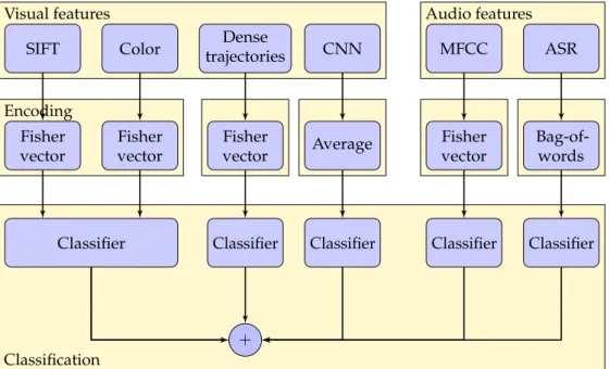
- SYSTEM DESCRIPTION 143 In addition to the visual features, we also extract features from the
- Localization
- RESULTS 145
- Results
- Classification results
- RESULTS 147
- Localization results
- CONCLUSION 151
- Conclusion
Compared to the experiments in Chapter3, we complement the motion-based features with several new features (see FigureA.1 for a summary illustration of the classification system). As negatives, we use (i) all examples of other classes from the Train part of the data, (ii) all uncropped videos in the background part of the data, (iii) all uncropped videos from other classes in the Validation part of the data, and (iv) all truncated examples of other classes in the Validation part of the data.