HAL Id: hal-00742039
https://hal.archives-ouvertes.fr/hal-00742039v2
Submitted on 11 Sep 2013
HAL is a multi-disciplinary open access archive for the deposit and dissemination of sci- entific research documents, whether they are pub- lished or not. The documents may come from teaching and research institutions in France or
L’archive ouverte pluridisciplinaire HAL, est destinée au dépôt et à la diffusion de documents scientifiques de niveau recherche, publiés ou non, émanant des établissements d’enseignement et de recherche français ou étrangers, des laboratoires
Energy saving in railway timetabling: A bi-objective evolutionary approach for computing alternative
running times
Rémy Chevrier, Paola Pellegrini, Joaquin Rodriguez
To cite this version:
Rémy Chevrier, Paola Pellegrini, Joaquin Rodriguez. Energy saving in railway timetabling: A bi- objective evolutionary approach for computing alternative running times. Transportation research.
Part C, Emerging technologies, Elsevier, 2013, 37, pp.20–41. �hal-00742039v2�
Energy saving in railway timetabling:
A bi-objective evolutionary approach for computing alternative running times
R´emy Chevrier∗, Paola Pellegrini, Joaqu´ın Rodriguez
Universit´e Lille Nord de France, IFSTTAR – ESTAS 20 rue ´Elis´ee Reclus, 59650 Villeneuve d’Ascq, France
Abstract
The timetabling step in railway planning is based on the estimation of the running times. Usually, they are estimated as the shortest running time increased of a short time supplement. Estimating the running time amounts to define the speed profile which indicates the speed that the train driver must hold at each position. The approach proposed in this paper produces a set of solutions optimizing both the running time and energy consumption.
The approach is based on an original method of speed profiling performed by a multi-objective evolutionary algorithm. The speed profiles found by the evolutionary algorithm are all compromises between running time on the one hand and energy consumption on the other hand. A set of results obtained on two lines are analyzed and discussed to highlight the relevance of such an approach in an practical context.
Key words: Running time, Energy saving, Railway timetabling, Multi-objective, Evolutionary algorithm, Optimization
1. Introduction
Over the years, the increase of traffic volumes in Western Europe and the increase of emission of pollutants have put a stronger and stronger accent
∗Corresponding author
Email addresses: remy.chevrier@ifsttar.fr(R´emy Chevrier),
paola.pellegrini@ifsttar.fr(Paola Pellegrini),joaquin.rodriguez@ifsttar.fr (Joaqu´ın Rodriguez)
on the development of more eco-aware transportation systems. A direct consequence is the search for a better management of energy. In railways, this better management may be sought, first of all, in the planning phase, during which the timetables are built.
All information required for the trips are computed during the planning phase. In particular, the train running times between stations are estimated during this phase to then compute notably the timetable of each train. Based on the timetable and the predefined running times, the energy-optimal train trajectories are computed offline and then communicated to the driver in a roadmap that he must follow [1]. The corresponding speed profiles precise the speed at each position on the track and they give also the switch-points indicating to the driver when changing the driving regime. In order to effi- ciently switching the regimes, the train drivers are trained and accustomed to the energy-efficient driving, notably by learning it under supervision in a train simulator.
As the timetabling process is based on the predefined running times be- tween stations, the definition of alternative running times will directly im- pact, of course, the traffic planning, but also the whole energy consumption.
Indeed, changing the running speed or the driving regimes that the train must hold to respect the time constraints, will modify the energy consumption and lead to have potentially energy-efficient timetables. Thus, the goal is to find energy-efficient speed profiles compliant to the requirements (signaling, time constraints) so that alternative timetables are possible.
The problem of speed-profiling has been addressed in the literature in several ways, taking energy into account or not, involving one or several objectives.
For optimizing energy efficiency of train operation, there exist methods searching for a single optimal solution minimizing energy consumption for a given running time. The problem can be solved with an analytical method calculating the sequence of optimal controls and change points such as in [2], or with switch-points and differential equations systems as explained in [1].
Furthermore, due to the critical aspects of real-time railway management, a body of work has been carried out to solve the optimal speed profile ac- cording to an available running time, such as in [3] or in [4] for multi-train scheduling. It is also possible to re-optimize the running times in real-time at network scale [5].
More recently, a method based on mixed integer linear programming has been proposed to optimize running times by using an objective function which
is a tradeoff between energy consumption and riding comfort [6].
Differently to most of the works, trajectory optimization can be addressed without optimal control theory, as in [7, 8] where the authors exploit the dynamic programming to solve the problem.
Most of the methods are designed to provide a single solution to the decision-makers, though they could need more flexibility in the timetabling process.
As far as we know, there are still few multi-objective approaches to opti- mize speed profiles. Differential Evolution [9] has been used for mass tran- sit systems [10] involving three objectives: punctuality, energy consumption and passenger comfort (by reducing jerks). Another evolutionary method has been developed to perform a speed-based model [11, 12], building speed profiles in a multi-objective way according to a set of predefined rules.
Although estimating the appropriate running time is crucial for the time- tabling process, in practice, the running times are usually based on the fastest journey multiplied by an arbitrary factor slightly greater than 1 to have a running time supplement [13]. In general, the time supplement allows the train driver to adapt the speed to the traffic. However, the time supplements can be reduced by relaxing the timetables of some specifications (tracks, platforms, time windows, ...) for reducing the use of railway capacity [14].
If perturbations occur, it may happen that the running times have to be modified to take conflicts or delays into account. In [15], the authors propose to forecast delays to produce a distribution of possible running times to be used when the timetable cannot be respected. The authors solve systems of linear differential equations to estimate possible running times.
The time supplement could also be used to save energy. Indeed, we can identify the most energy-friendly speed profile, which benefits of this addi- tional time for using energy-free driving regimes. The speed profile designed in this way differs from the one of the fastest journey in duration (longer) and energy consumption (weaker).
In this paper, we propose an original approach to compute train run- ning times by concurrently minimizing both energy consumption and run- ning time. Usually, the running time is estimated for an entire trip including a set of journeys between stations and the time supplement is spread over the trip [16]. However, as a preliminary work, we consider here the defini- tion of running time between two stations. Since a trip includes a succession of journeys from one station to another, the approach proposed performs a running time calculation of one journey. This calculation is done by building
the speed profile according to a set of rules that we propose to determine the order of driving regimes that the train driver must follow. In particular, a braking must not be followed by an acceleration, because it is absurd from an energy consumption point of view. Moreover, the approach under considera- tion must be capable of providing a set of tradeoff-solutions for the decision- makers in a single run. In such a way, they will be able to choose a running time adapted to their needs in the timetabling process. Thus, the paper deals with a bi-objective optimization of speed profiling with energy saving.
Given that evolutionary algorithms (EA) are well-suited to multi-objective optimization [17], our approach is based on a state-of-the-art multi-objective EA: the Indicator-Based Evolutionary Algorithm (IBEA) [18].
The paper is organized as follows. At first, Section 2 concerns the basic principles of train dynamics and running time calculation used in the opti- mization model. Then, Section 3 presents the problem under study and its formulation. The algorithms for building a speed profile and evaluating a solution are presented and detailed in Section 4. In Section 5, we present both the principles of multi-objective optimization and IBEA. The specific components of the algorithm are also presented in this section. Section 6 presents two case-studies (including one real railway line), as well as the re- sults of speed profile optimization obtained on these instances. Analysis and discussion are provided for highlighting the interest of such a method in the planning process. Finally, Section 7 concludes the paper.
2. Running times and train dynamics
In this section, we explain how the running times are calculated and we recall the basic formulas of train dynamics used to perform this calculation.
The reader can refer to [19, 20] to have a more detailed explanation of train dynamics. The formulas presented may be modified or replaced without changing the nature of optimization problem defined in the following. The model used here is an approximation of the reality. However, a more accurate model implying, for example, to consider the length of the train, the cars and their positions on the track, but also the axles and the wheels, requires to develop a more precise railway dynamics model.
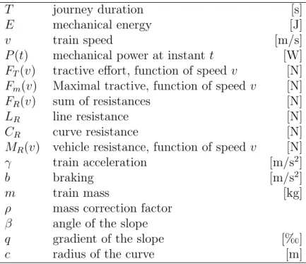
Table 1 summarizes the main symbols used in the paper.
Table 1: Definition of the symbols used in train dynamics
T journey duration [s]
E mechanical energy [J]
v train speed [m/s]
P(t) mechanical power at instant t [W]
FT(v) tractive effort, function of speedv [N]
Fm(v) Maximal tractive, function of speedv [N]
FR(v) sum of resistances [N]
LR line resistance [N]
CR curve resistance [N]
MR(v) vehicle resistance, function of speedv [N]
γ train acceleration [m/s2]
b braking [m/s2]
m train mass [kg]
ρ mass correction factor β angle of the slope
q gradient of the slope [‰]
c radius of the curve [m]
2.1. Setting sequences of driving regimes
In order to define accurate running times, it is necessary to build speed profiles, which are indicated in the roadmaps that the train driver must follow. According to the theory of optimal control, there are four optimal regimes defined by application of the Maximum Principle (see [21, 1] for details): Acceleration at full power; Cruising at constant speed; Coasting (inertia motion while the engine is stopped); Maximum braking (according to the service braking, softer than emergency braking). Since acceleration is very energy-consuming, the inefficiency of applying unnecessary sequences of braking followed by acceleration is straightforward. Hence, it is a principle of the method that we propose in the paper. In the roadmaps to provide to the drivers, a braking must not be followed by an acceleration.
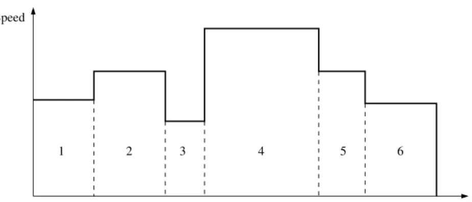
The problem we deal with consists in designing the most suited speed profile over the track. This track is composed of a sequence of sections, in which the speed has to be tuned. A section is defined by a length and a constant and fixed maximal speed. Consecutive sections always have different
maximal speed (see Fig. 1).
Speed
4
1 3 5 6
Position 2
Figure 1: Decomposition of the track according to the maximal speeds
In principle, a one-section journey can be divided in four steps as depicted in Fig. 2 (we assume there is neither slope nor curve in this example). Let vm be the maximal speed. First, the train accelerates (A) in order to reach speed vm as quickly as possible. Then, a cruising phase (Cr) follows during which the acceleration is nil and the traction effort equals the resistance to the train advance. Given that the wheel/rail adhesion is weak, it is common to let the train coast over long distances [22, 23], e.g. points Co(1), Co(2) indicate two positions from which coasting can be started. Coasting from point Co(1) may increase the journey duration a little while reducing the use of mechanical energy. By coasting from point Co(2), the energy consumption may be further decreased with a consequent increase of journey duration.
The sooner the coasting starts, the greater the economy, but the longer the journey duration. Point Co(0) indicates the last position from which the train can brake with its normal service braking (B) for being able to stop at the end of the section.
2.2. Elements of railway dynamics
The fundamental equation of dynamics states the relation between the forces FT, FR, speed v, mass m and acceleration γ:
FT(v)−FR(v) =ρ m γ, (1)
ρ being a mass correction factor usually set to ρ= 1.04 [23, 1].
Co(2) m
Speed
Position Co(1) Co(0) v
0 A
Cr
Co
B
Figure 2: Usual speed profile over one section in four steps (assuming no slope): acceler- ation (A), cruising (Cr), coasting (Co) and Braking (B).
2.2.1. Tractive effort
Tractive effortFT is the effort that the train produces for running, bounded by the maximum tractive effortFm. The maximum tractive effort that a train can produce is a function of both the train characteristics and the current speed.
2.2.2. Constraints
Train’s speed, tractive effort and braking are bounded. Let vcm be the maximum speed of trainc,Fm(v) the maximum tractive effort that the train can exert when traveling at speed v, and bm the maximum service braking.
v ≤ vmc (2)
FT(v) ≤ Fm(v) (3)
b ≤ bm. (4)
Given that the deceleration depends also on the gradient of the track, it may happen that using the maximum service braking bm is not sufficient to slowdown the train if it runs in a steep descent. The respective effect in acceleration may appear if the train runs in a climb so steep that it cannot accelerate though using the maximum tractive effort Fm(v). However, such gradients are unusual in practice, given that the tracks are designed in such a way that the rolling stocks can move without difficulty. The problem may appear with materials not planned to run on some tracks.
2.2.3. Resistances
The resistance to the train advance FR corresponds to the sum of line (LR), curve (CR) and vehicle (MR) resistances:
FR(v) =LR+CR+MR(v). (5)
Line resistanceLR depends on the train mass and the slope angle β:
LR=m g sinβ, (6)
g being the gravity constant: g = 9.81 N/kg. However, line resistance LR is often approximated as:
LR=m g q, (7)
with q = tanβ. This is considered a good approximation since, for small values of β as the ones considered, sinβ and tanβ are very similar. The quantity q is a gradient measured in meters per thousand.
Concerning curve resistance, the value of CR is approximated by CR=m g 700
c . (8)
Finally, vehicle resistance MR combines both rolling resistance and air resistance. The former linearly increases as a function of the adhesion and the wheel rims. The latter quadratically increases as a function of the train velocity. Resistance MR depends on the physical properties of the train and its current speed. In order to simplify its calculation, we use the Davis’ equa- tion [24] proposed in the 1920s and still used today. This formula introduces constantsA, BandC, specific to the rolling stock, and allows to approximate the vehicle resistance MR as follows:
MR(v) =A+Bv+Cv2. (9)
2.2.4. Mechanical energy consumption
Let E be the mechanical energy needed to move the train. It can be calculated as the integral of the mechanical power over the running time T [1]. For convenience, let F(t) and v(t) be the tractive effort and the train’s speed at instant t, respectively:
E = Z T
0
P(t) dt with P(t) =F(t) v(t). (10)
PowerP(t) generated by the train at instanttis calculated in function of the regime adopted, within functionapply regime (Algorithm 1 in Section 4.1).
If we want to consider aspects as electrical-mechanical energy conversion (for instance, motors and inverters), it is possible to use another railway dynamic model including the principles mentioned. In no case, the opti- mization model will be affected because it uses the objective values T, E.
However, changing the dynamic model will impact the objective value E, and consequently the speed profiles generated.
2.3. Description of the driving regimes
As mentioned in Section 2.1, according to the Maximum Principle, four regimes can be adopted by the train, when power recovery (regenerative braking) is not used [8]: acceleration, cruising phase, coasting and braking.
Energy consumption and running time evolve differently during each of them.
As mentioned by Miyatake and Ko in [8], there are difficulties in effi- cient utilization of regenerative braking. In particular, an accelerating train must be close to the braking one so that the former can absorb the regener- ative energy. However, only one train is actually considered in our method, whereas the problem of recovering energy by another train is relevant when considering several trains at once. Moreover, such a problem implies the optimization of the synchronization of the trains in the construction of the timetable, which is out of the scope of the paper. Hence, we do not consider the regenerative braking.
2.3.1. Acceleration
During this phase, the train accelerates at full power. The delivered power, P, depends on both tractive effort FT and speed v. Hence, during an acceleration:
FT(v) = Fm(v) (11)
P(v) = FT(v)v. (12)
2.3.2. Cruising phase
This regime consists in maintaining the speed constant, i.e., the accelera- tion is nil: γ = 0. In fact, the resistance is counterbalanced by the minimum necessary tractive effort: FT(v) = FR(v). In other words, the train must adapt its effort to the resistance either by partially braking or producing an effort according to the gradient and the resistances (line and vehicle).
Sinceγ results from both the acceleration due to the forces of motion and the braking, we denote a the acceleration due to the forces of motion and b the service braking, so that: γ =a−b.
Letσ be the gradient representing the threshold under which the descent may allow the train to accelerate without effort. We can formalize the effort in the two cases defined below.
1. If q ≥ σ, the train has to produce effort to maintain the speed. First, we determine the resistance FR(v) and then we set the tractive effort FT(v) that the train should exert to counterbalance FR(v)≥0:
FT(v) = FR(v) ⇔ γ = 0. (13)
Last but not least, the power delivered can be deduced as follows:
P(v) = FT(v) v. (14)
2. If q < σ, the train has to partially brake to maintain the speed. First, we state resistance FR(v). Given that FR(v) < 0 in this case, we determine the resulting acceleration a > 0 to deduce the braking b necessary to keep γ =a−b = 0.
b =a= −FR(v)
ρ m . (15)
Finally, as no power recovery is considered, we set the power delivered as nil:
P(v) = 0. (16)
2.3.3. Coasting
The coasting corresponds to an inertia motion, while the engine is stopped.
The tractive effort is therefore nil:
FT(v) = 0. (17)
As a consequence, the energy consumption during coasting is nil andP(v) = 0.
2.3.4. Braking
The braking is computed using the maximum service brakingbm. When braking, the tractive effort is therefore nil:
FT(v) = 0. (18)
Like in the coasting regime, the energy consumption during coasting is nil and P(v) = 0.
Table 2: Symbols used in the problem definition
S sequence of sections composing the train path n number of sections
i section index: 1≤i≤n pi starting position of section i
with respect to a reference point li length of section i
vm,i maximum speed in section i
(remark that vm,i>0 for all i= 1, ..., n) lf,i length of the first part of section i ls,i length of the second part of section i tf,i duration of the first part of section i ts,i duration of the second part of section i ef,i energy spent in the first part of section i es,i energy spent in the second part of section i
3. Problem definition
In order to build a speed profile between two stations, we build the speed profile within each section covered by the train, sequentially. Each section is then decomposed according to a set of speeds for choosing the appropriate driving regimes. The main symbols used in the following are defined in Table 2.
3.1. Objectives formulation
The problem under study can be formulated as a set Φ of two objective functions to be minimized while respecting constraints. The first objective function represents the minimization of journey duration T, and the second the reduction of energy consumption E.
Φ = (minT,minE). (19)
Objective values (Tu, Eu) of solutionuare assessed byeval solution, which is a function defined by Algorithm 3 in Section 4.2.
3.2. Speed-based decomposition of a section 3.2.1. Using target-speeds as decision variables
As the train path is decomposed into a set ofnsections, the speed profile is successively built in each section. This construction is based on the use of target-speeds, which allow the decomposition of each section into a sequence of driving regimes. For each sectioni= 1, ..., nwe define the following speeds:
ve,i, vx,i, va,i, vb,i ∈ R. The speedsve,i and vx,i are, respectively, the entrance and exit speeds of sectioniand they are determined while building the speed profile.
The speedsva,i, vb,iare the decision variables searched for by the algorithm and they are at the basis of the decomposition of the section. They represent two speed-levels that the train must reach while running over the section.
The main idea is to allow the introduction of driving regimes following a set of rules which depend on the speeds, as explained in the following.
3.2.2. Principle of decomposition of a section
Speed profiling is done in two phases, each depending on a set of speeds.
Figure 3 depicts the decomposition of the speed profile over one single section, as well as the corresponding time-position diagram. The main idea consists in splitting the section into two parts: a first part in which the acceleration at full power (the most energy-consuming driving regime) can be used and a second part for using energy-friendly (cruising) or energy-free (coasting, braking) driving regimes.
During the first part, the train enters at speed ve,i and has to reach the first target-speed va,i by braking or accelerating. Then, during the second part, the train tries to reach speed vb,i, initially by coasting. Additional regimes may be used to reach speed vb,i (braking) and complete the rest of the section (cruising). Even if some of these driving regimes are not used, globally, their use follows the order: coasting, cruising, braking. Building the profile between the entrance speed ve,i and the first target-speed va,i allows the identification of the length and the time necessary for the first part: lf,i and tf,i, respectively. This building also allows the deduction the length of the second part of the section: ls,i = li −lf,i. The construction of the second part starts from position pi +lf,i and depends on target-speeds va,i and vb,i. The produced sequence of driving regimes leads to determine the exit speed vx,i of section i and, obviously, ve,i+1 =vx,i, i < n. The details of the construction are explained right below.
B
f,i ts,i
lf,i ls,i
Time position diagram
vb,i va,i
A
Co Cr
t
0 Position
Speed
Position Time
0
First part
First part Second part Second part Speed profile
Figure 3: Decomposition of a section into two parts: (a) Speed profile describing the sequence of the driving regimes according to the target-speeds; (b) Time position diagram describing the corresponding train path as well as the required times to cover the section.
Constraints. During the solution construction, we impose Constraints (20) to (22) to the decision variables for each section.
va,i ≥ vb,i ∀i= 1, ..., n (20)
vm,i ≥ va,i ∀i= 1, ..., n (21)
vb,i > 0 ∀i= 1, ..., n (22)
As explained in the following, the value of vb,i, i= 1, ..., n, may be changed during the evaluation of the objective function, in case the original one results unfeasible.
4. Solution assessment and running time calculation
In this section, the algorithms for building the speed profile and for assess- ing a solution are given and detailed. But, beforehand, we provide algorithms
for calculating train dynamics corresponding to a driving regime. These al- gorithms are essential to compute distance covered, energy consumed and time spent during a driving regime. After this description, we will give the algorithms of speed profiling as a function of the target-speeds defined in each section. In the following, symbols ac, cr, co, br, respectively, represent acceleration, cruising, coasting and braking.
4.1. Calculation of driving regime
Based on the description of the possible driving regimes, Algorithm 1 defines function apply regime which calculates time spent, length, energy, and speed at each position in function of the characteristics of the track and the train, and also of the speeds given in input. The principle at the basis of this iterative function is to determine efforts, resistances, acceleration, speed, power and energy at each instant t (let ∆t be the time-slot).
Since functionapply regime needs to be interrupted when changing the driving regime, function end reached(Algorithm 2) indicates when the cur- rent regime is implemented. The main reasons to interrupt a regime are either that the target-speed is reached or that the limit position beyond which the regime used must be changed is attained.
4.2. Objectives computation
For computingT and E, we apply the functioneval solutiondescribed in Algorithm 3. Within this function,T andE are calculated for each section consecutively by the function eval section defined in Section 3.2.
Algorithm 4 describes the function named eval section. Based on the characteristics of a section and the values of the decision variables, this func- tion returns the time and the energy spent in the section itself. Within this function, we use two additional sub-functions first partandsecond part, which respectively build the speed profile on the first and the second part of the section under consideration (Algorithms 5 and 6 respectively).
Construction of the speed profile in the first part. The first part corresponds to the entrance in the section and depends on two speeds: the entrance speed ve,iand the target-speed va,i. The latter is a decision variable of the problem and it is searched for by the evolutionary algorithm. The construction of the speed profile is carried out through Algorithm 5, which identifies the regime to be used: acceleration if va,i > ve,i, braking otherwise. If the two speeds are equal (ve,i = va,i), length, time and energy spent are nil: lf,i = 0, tf,i = 0, ef,i= 0; function end reached() returns 1 in such a case.
Algorithm 1: Function apply regime(v1, v2, l, p, r)
Data:v1: initial speed,v2: speed to reach,l: distance to cover,p: start position,r: driving regime to use
Result: (t, l, e, R): a vector containing the time spent, the length and the energy used during the motion. Ris a vector containing the pairs (pt, vt).
Initialization t=h;l, e= 0;R= () vt=v1;pt=p begin
whilenot end reached(vt,v1,v2,p,p+l,r)do
CalculatingLR, CR, MRas function ofvt, pt(Eq. 7, 8, 9) FR=LR+CR+MR
if r =={brorco}then FT = 0
if r ==br then b=bm
else b= 0 else
if r == crthen
FT = max(0,min(Fm, FR)) b= max(0,−FR/ρ.m) else– –r== ac
FT =Fm
b= 0 a=FTρ m−FR+b vt=vt+a∆t pt=pt+vt∆t l=l+vt∆t e=e+FTvt∆t R=R∪(pt, vt) t=t+ ∆t end
Construction of the speed profile in the second part. This part depends on both variables defined for section i, namely va,i and vb,i and it depends on the gradient, the maximum speed of the following section and the capability to coast all over lengthls,i. Letlcobe the length of coasting,lcr the length of cruising, lbr the length of braking. Algorithm 6 describes the construction of the second part. It has to be noted that two additional functions are used in the algorithm. The first is search for intersection which computes the changing between two regimes by searching for the intersection of the speed curves representing the driving regimes under consideration. The second is apply reverse regime which is the counterpart of apply regime but it
Algorithm 2: Function end reached(v1,v2,p1, p2, r)
Data:v1: current speed,v2: target-speed,p1: current position,p2: limit position,r: current driving regime
Result:reached={0|1}
begin
reached = 1;
switchrdo casebr
if v1> v2 orp1< p2 thenreached = 0 caseco
if v1< v2 orp1< p2 thenreached = 0 casecr
if p1< p2thenreached = 0 caseac
if v1< v2 orp1< p2 thenreached = 0 end
Algorithm 3: eval solution(u= (va,1, vb,1, ..., va,n, vb,n)).
Data: for each sectioni= 1, ..., n:va,i, vb,i, pi, li, vm,i
Result: vector (T , E) including the total running time and total energy consumption (T , E) = (0,0);
(T , E) = (T, E)+eval section(0,va,1,vb,1,va,2,p1,l1,vm,1,vm,2);
fori= 2, ..., n−1do
(T , E) = (T , E)+eval section(min{vb,i−1, vm,i},va,i,vb,i,va,i+1,pi,li,vm,i,vm,i+1);
(T , E) = (T, E)+eval section(min{vb,n−1, vm,n},va,n,vb,n, 0,pn,ln,vm,n, 0)
Algorithm 4: eval section(ve, va, vb, p, l, vm, vn)
Data:ve: entry speed,va: target speed in the first part,vb: target speed in the second part,p:
entry position,l: section length,vm: maximum speed of the section,vn: maximum speed of the next section
Result: vector (t, e) including the total running time and total energy consumption in the section begin
1
(ta, la, ea, Ra) = first part(ve, va, l, p) ; 2
(tco, tcr, tbr, eco, ecr, ebr, lco, lcr, lbr, Rco, Rcr, Rbr) = second part(va, vb, p, la, vm, vn) ; 3
t=ta+tco+tbr+tcr; 4
e=ea+eco+ebr+ecr; 5
end 6
computes the phase from the end-point to the beginning. This function is used when no beginning-point is known for the driving regime to use, but the end-point of the phase is known. Given that these two functions can be retrieved easily, they are not defined in this paper.
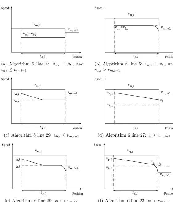
If va,i = vb,i, the speed profile consists of a cruising phase at speed va,i all along the section if vm,i+1 ≥ va,i (Fig. 4(a)), i.e., if the maximum speed
Algorithm 5: first part(ve, va, l, p)
Data:ve: entry speed,va: target speed in the first part,p: start position,l: section length,vm: maximum speed of the section
Result: vector (ta, la, ea, Ra) including the total running time, length, energy consumption and regime used in the section.
begin 1
ifve< vathen 2
(ta, la, ea, Ra)=apply regime(ve,va,l,p,ac) ; 3
else 4
(ta, la, ea, Ra)=apply regime(ve,va,l,p,br) ; 5
end 6
of the following section is higher than the current target-speed. Otherwise it consists in a cruising phase at speedva,ifollowed by a braking to reach speed vm,i+1 (Fig. 4(b)).
Letvl be the last speed measured at the end of the coasting and returned by function exit coast (not defined in the paper). If va,i > vb,i, we try to insert a coasting phase:
• Ifq ≥σ the train decelerates by coasting, and thusvl < va,ibecause of the slowdown due to the resistive efforts while coasting,
• If q < σ: there is a steep descent.
If the coasting permits to reach vb,i, then vl = vb,i. Otherwise, a number of cases must be distinguised to be treated differently. When vl < va,i, we distinguish four cases depending on the possibility to coast along a distance smaller than or equal to the distance ls,i:
• if vb,i ≤vm,i+1
i. if the train may reach speed vb,i, starting at speed va,i, by coast- ing along the length ls,i, the speed profile includes the coasting followed by a cruising regime at speed vb,i in the remaining dis- tance (Fig. 4(c)). The exit speed vx,i equals vb,i,
ii. if the train covers the section by coasting and it never reaches speedvb,i, then we set: vb,i =vl(Fig. 4(d)). In addition,vx,i =vb,i.
• if vb,i > vm,i+1
iii. if the train may reach speedvb,i, starting at speedva,i, by coasting along the length ls,i, the same speed profile described in (i) is
imposed, but a final braking is necessary to enter the following section at speedvm,i+1 (Fig. 4(e)). In this case,vx,i =vm,i+1, iv. if the train covers the second part of the section by coasting and
it never reaches speed vb,i, then a final braking is imposed for attaining this speed (Fig. 4(f)). Let vc be the speed measured when starting braking, i.e., vc is obtained after calling function search for intersection. Since speed vb,i cannot be attained, it is then corrected by replacing its value with: vb,i = vc. Last, vx,i =vm,i+1.
As discussed above, it may happen that a coasting results in an acceler- ation if q < σ, in this case:
• if vb,i ≤ vm,i+1, the coasting is interrupted by a braking to leave the section at speed vb,i (Fig. 5(a)),
• if vb,i > vm,i+1, the train stops coasting and brakes to leave the section at speed vm,i+1. Speedvb,i is therefore corrected tovm,i+1: vb,i =vm,i+1 (Fig. 5(b)).
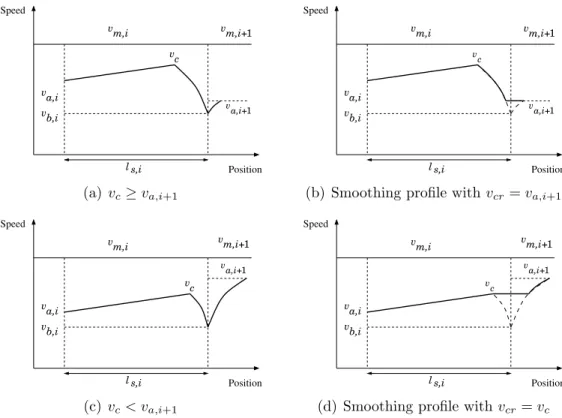
4.3. Post processing: smoothing the speed profiles
Although the construction of speed profiles aims to avoid sequences com- posed of braking followed by acceleration, a post-processing is necessary for guaranteeing that it is always the case. In fact, if the slope in the second part of the section is sufficiently steep to make the train accelerate while coasting, then a braking is introduced to reach speed vb,i. If vb,i < vm,i+1, this braking could be followed by an acceleration (if va,i+1 > vb,i).
For avoiding this, we use a smoothing post-processing to eliminate two types of sequences: (Braking, Acceleration at full power); (Braking, Accel- eration while coasting). Whatever the sequence under consideration, we can distinguish two cases for which we determine a cruising phase replacing one part of the sequence depending on speedsvc(defined as speed measured when starting braking) and va,i+1 (Fig. 6(a, c)). The cruising speed corresponds to the minimum between them: min(vc, va,i+1). Finally, Figures 6(c, d) are respectively the smoothed profiles of Figures 6(b, d).
All along this inserted cruising phase, it is necessary to compute the effort necessary to maintain the speed constant. This effort will replace the one previously computed for the acceleration phase in the evaluation of
Algorithm 6: second part(va, vb, p, l, vm, vn)
Data:va: target speed in the first part,vb: target speed in the second part,p: start position,l:
section length,vm: maximum speed of the section,vn: maximum speed of the next section Result: vector (tco, tcr, tbr, eco, ecr, ebr, lco, lcr, lbr, Rco, Rcr, Rbr) including the total running
time, the total energy consumption and the total run length of each regime used in the second part of the section.
begin 1
if va==vbthen 2
if va< vnthen 3
(tcr, lcr, ecr, Rcr)=apply regime(va,vb,l−la,p+la,cr) ; 4
else 5
(tbr, lbr, ebr, Rbr)=apply reverse regime(vb,vn,l−la,p+l,br) ; 6
(tcr, lcr, ecr, Rcr)=apply regime(va,vb,l−la−lbr,p+la,cr);
7
else 8
//va> vb
9
vl= exit coast(va,vb,l−la,p+la);
10
(tco, lco, eco, Rco)=apply regime(va,vb,l−la,p+la,co);
11
if vl> vathen 12
if vn≤vbthen 13
(tbr, lbr, ebr, Rbr)=apply reverse regime(vm,vn,l−la,p+l,br) ; 14
(tco, tbr, lbr, lco, eco, ebr, Rbr, Rco)= search for intersection(Rco,Rbr) ; 15
vb=vn; 16
else 17
(tbr, lbr, ebr, Rbr)=apply reverse regime(vm,vb,l−la,p+l,br) ; 18
(tco, tbr, lco, lbr, eco, ebr, Rco, Rbr)= search for intersection(Rco,Rbr) ; 19
else 20
if vl> vbthen 21
if vn≤vlthen 22
(tbr, lbr, ebr, Rbr)=apply reverse regime(vm,vn,l−la,p+l,br) ; 23
(Rco, Rbr, vc)= search for intersection(Rco,Rbr) ; 24
vb=vc
25
else 26
vb=vl; 27
else 28
vt= min(vb, vn) ; 29
(tbr, lbr, ebr, Rbr)=apply reverse regime(vb,vt,l−la,p+l,br) ; 30
(tcr, lcr, ecr, Rcr)=apply regime(vb,vb,l−la−lco−lbr,p+l,cr);
31
t=ta+tco+tbr+tcr; 32
e=ea+eco+ebr+ecr; 33
end 34
the second objective of the optimization. The same holds for the running time associated to the speed profile. The advantage of inserting a cruising phase instead of an inappropriate sequence is to reduce the journey duration while also reducing the quantity of energy consumed, because acceleration is replaced by a regime far less energy-consuming.
It has to be noted that the post processing is applied to any solution as
s,i Speed
Position l
vm,i+
v
1 m,i
= vb,i va,i
(a) Algorithm 6 line 4: va,i = vb,i and va,i≤vm,i+1
l s,i Speed
Position
v vm,i+1
vm,i
= vb,i a,i
(b) Algorithm 6 line 6: va,i = vb,i and va,i > vm,i+1
l s,i Speed
Position b,i
m,i+1 v vm,i
va,i v
(c) Algorithm 6 line 29: vb,i≤vm,i+1
l s,i Speed
Position b,i
l m,i+1 v vm,i
va,i
v
v
(d) Algorithm 6 line 27: vl≤vm,i+1
l s,i Speed
Position
b,i vm,i+1
vm,i
va,i v
(e) Algorithm 6 line 29: vb,i> vm,i+1
l s,i
vl Speed
Position c
m,i+1 v vm,i
va,i
vb,i
v
(f) Algorithm 6 line 23: vl> vm,i+1
Figure 4: Description of the possible situations in the second part of a section
soon as it is generated.
l s,i
vl vc Speed
Position m,i
va,i vb,i
vm,i+1 v
(a) Algorithm 6 line 18
l s,i
vl vc Speed
Position m,i
va,i v v
b,i m,i+1
v
(b) Algorithm 6 line 14
Figure 5: Description of particular situations in the second part of a section, when gradient qis negative and the descent is such that a train can accelerate without effort.
l s,i
va,i+1 Speed
Position m,i+
m,i
va,i vb,i
vc v 1 v
(a) vc≥va,i+1
l s,i
va,i+1 Speed
Position vm,i 1
va,i vb,i
vm,i+
vc
(b) Smoothing profile withvcr=va,i+1
l s,i
va,i+1 Speed
Position m,i m,i+
va,i vb,i
vc v 1 v
(c) vc < va,i+1
l s,i
va,i+1 Speed
Position vm,i 1
va,i vb,i
vm,i+
vc
(d) Smoothing profile withvcr=vc
Figure 6: Description of smoothing of speed profiles: profiles (a) and (b) have a braking followed by an acceleration (at full power or by coasting in descent); profiles (c) and (d) are the respective smoothed speed profiles.
5. Evolutionary Multi-objective Optimization
The problem under study is a multi-objective continuous optimization
this kind of algorithm is known to be well-suited to multi-objective problems [17]. First, we present multi-objective optimization principles and concepts.
Then, we introduce the state-of-the-art evolutionary algorithm which is used in the experimental analysis. Finally, we present the mechanisms specific to our application.
5.1. Multi-objective Optimization
A general Multi-objective Optimization Problem (MOP) can be defined by a set of k objective functions f = (f1, f2, . . . , fk) and a set U of feasible solutions in the decision space. Let Z be the objective space Z = f(U).
Without loss of generality, we assume here that each objective function is to be minimized. To each solution u∈U is assigned an objective vector z ∈Z withz ={z1, z2, ..., zk}computed on the basis of the vector functionf :U → Z with z = f(u) = (f1(u), f2(u), . . . , fk(u)). An objective vector z ∈ Z is said todominate another objective vectorz0 ∈Ziff ∀i∈ {1,2, . . . , k},zi ≤zi0 and ∃j ∈ {1,2, . . . , k} such thatzj < zj0. A decision vector u∈U dominates a decision vectoru0 ∈U iff(u) dominatesf(u0). An objective vectorz ∈Zis said to benon-dominated iff no other objective vectorz0 ∈Z exists such that z0 dominatesz. A solution u∈U is said to beefficient, orPareto optimal, if its mapping in the objective space results in a non-dominated point.
Due to the complexity of the underlying problem, the overall goal is of- ten to identify a good approximation of the efficient set. Population-based metaheuristics in general, and evolutionary algorithms in particular, are com- monly used to this end, as they are capable of finding multiple and well-spread non-dominated solutions in a single run [17].
5.2. Indicator Based Evolutionary Multi-objective Algorithm
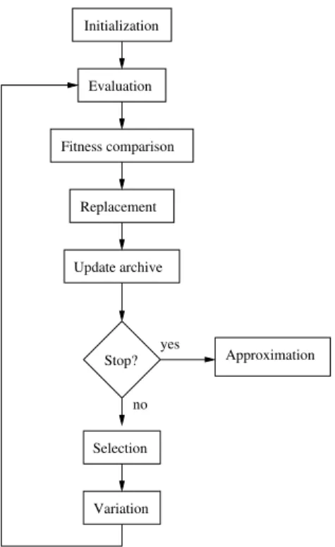
Over the last decades, a very large number of evolutionary algorithms for MOP solving have been proposed in the literature [17, 25]. These approaches can be seen as frameworks in which problem-related components have to be defined. In this work, we have used a state-of-the-art evolutionary multi- objective optimization algorithm, namely the Indicator-Based Evolutionary Algorithm (IBEA) [18]. This algorithm follows the main steps illustrated in the flowchart of Fig. 7.
IBEA characterizes the trend in evolutionary computation dealing with indicator-based search which has become popular over recent years. The main idea is to introduce a total order between solutions by means of a binary quality indicator. In multi-objective optimization, ‘quality’ represents
no Initialization
Evaluation
Fitness comparison
Replacement
Update archive
Stop?
Selection
Variation
Approximation yes
Figure 7: Flowchart of an evolutionary multi-objective optimization algorithm.
the well-spread aspect of the solutions in a front. Each solution contributes to the spread of the front, and hence to its quality [18].
The fitness assignment scheme is based on a pairwise comparison of so- lutions from the current population with regard to the indicator I+ [26].
To each individual u is assigned a fitness value φ(u) which is to be max- imized, and measuring the contribution of the solution u and hence the
‘loss in quality’ if u is removed from the current population Q, i.e., φ(u) = P
u0∈Q\{u}(−e−I(u0,u)/κ), where κ >0 is a user-defined scaling factor.
The variation step comprises recombination (crossover) and mutation.
The selection for crossover consists of a binary tournament between randomly chosen individuals and the selection for replacement consists in iteratively removing the worst solution from the current population until the required population size is reached. The fitness information of the remaining individ- uals is updated whenever one is deleted. Moreover, all new non-dominated solutions found during the process are archived in a separate population.
This archived population is updated every iteration in function of the new
non-dominated solutions for discarding the dominated ones.
5.3. Solution representation and initialization
A solution is defined by a vector of speeds: hva,1 vb,1 ... va,n vb,ni. Given that two speeds are necessary to represent a section, the number of compo- nents of solution u equals twice the number n of sections: #u= 2n.
To avoid too many unfeasible solutions at the beginning of the optimiza- tion, a specific initialization strategy is developed based on the fastest jour- ney, as described in Section 5.3.2.
5.3.1. Determination of the reference solution
In order to have a reference solution for further comparisons, we search for the solution which minimizes the running time, denoted u∗. Concretely, it consists in driving as fast as possible with respect to the speed constraints of the track.
A complete description of this calculation is given in [20]. In few words, the speed profile is built in three steps. First, the method consists in de- termining all necessary braking at the end of the sections for respecting the maximal speed of consecutive sections. Second, it consists in determining the maximal acceleration at the beginning of each section. Third, cruising phases are added between accelerations and brakings to complete the speed profile. The obtained solution represents the lower-bound T of running time and serves also as basis of comparison for the energy consumption. The decision-maker will be able to limit the possible range of running time by upper-bounding it to a duration equal to x×T, by setting parameterx >1.
5.3.2. Initialization of the population
The solutions are based on solution u∗ and are successively initialized.
The initial population as well as the following ones are composed of a fixed number N of solutions. Within each initialization of solution µ ∈ [1, N], the values of vµa,i, vb,iµ are determined from vua,i∗, vb,iu∗ in such a way that the solution initialized is automatically longer and less energy-consuming than the reference solution u∗. At every solution initialization, the solution is longer than the previous one. In our implementation, we have chosen a very easy way to do this. First, we assume that the population is limited to 50 solutions: N = 50. Then, the interval Ii for decreasing speeds vµa,i, vb,iµ per