[PENDING] Théorie spectrale et de la diffusion pour les réseaux cristallins

(1)

HAL Id: tel-01501943

https://tel.archives-ouvertes.fr/tel-01501943

Submitted on 4 Apr 2017

HAL is a multi-disciplinary open access archive for the deposit and dissemination of sci- entific research documents, whether they are pub- lished or not. The documents may come from teaching and research institutions in France or abroad, or from public or private research centers.

L’archive ouverte pluridisciplinaire HAL, est destinée au dépôt et à la diffusion de documents scientifiques de niveau recherche, publiés ou non, émanant des établissements d’enseignement et de recherche français ou étrangers, des laboratoires publics ou privés.

cristallins

Daniel Alejandro Parra Vogel

To cite this version:

Daniel Alejandro Parra Vogel. Théorie spectrale et de la diffusion pour les réseaux cristallins. Mathé- matique discrète [cs.DM]. Université de Lyon, 2017. Français. �NNT : 2017LYSE1001�. �tel-01501943�

(2)

N^o d’ordre NNT : 2017LYSE1001

THÈSE DE DOCTORAT DE L’UNIVERSITÉ DE LYON

opérée au sein de

l’Université Claude Bernard Lyon 1 École Doctorale Infomaths ED512

Spécialité : Mathématiques

Soutenue publiquement le 09/01/2017, par :

Daniel Alejandro Parra Vogel

Théorie spectrale et de la diﬀusion pour les réseaux cristallins

Devant le jury composé de :

M. KELLENDONK Johannes, Professeur des Universités, Université Lyon 1 Président Mme ANNÉ Colette, Chargée de Recherche - HDR, Université de Nantes Examinatrice M. FAUPIN Jérémy, Professeur des Universités, Université de Lorraine Rapporteur M. HÄFNER Diertrich, Professeur des Universités, Université de Grenoble Examinateur Mme TRUC Françoise, Maître de Conférences - HDR, Université de Grenoble Examinatrice M. RICHARD Serge, Maître de Conférences - HDR, Université Lyon 1 Directeur de thèse

(3)

(4)

Résumé de la thèse

Dans cette thèse nous nous intéressons à différents aspects de la théorie spectrale et de la diffusion pour des opérateurs qui agissent sur des espaces discrets. Ces opérateurs sont les analogues discrets des opérateurs différentiels sur des variétés Rie- manniennes pour le Chapitre 1 et Chapitre 2, et des opérateurs pseudodifférentiels magnétiques surR^d dans le Chapitre 3.

Dans le Chapitre 1 nous étudions des opérateurs de Schrödinger périodiques sur des cristaux topologiques ainsi que leurs perturbations. Les cristaux topologiques sont une version abstraite de graphes périodiques qui permettent de modéliser des cristaux parfaits. Ils sont donnés par un recouvrement d’un graphe fini X par un graphe infini X tel que X admet un action de Z^d compatible avec le recouvrement. Nous sommes donc amenés à étudier des opérateurs de Schrödinger périodiques de la forme H₀ = Δ +V surX, où l’opérateur Δ correspond au Laplacien discret périodique sur X etV est un potentiel périodique. Le Laplacien périodique est défini une fois qu’on a choisi une mesuremsurX périodique par rapport à l’action deZ^d. Ce cadre permet d’étudier deux types de perturbations. D’un côté, on peut modifier la mesure par une mesurem non périodique, et d’un autre côté on peut aussi remplacer le potentiel par un potentiel non périodique V. En utilisant la méthode de l’opérateur conjugué, on démontre, sous certaines conditions de convergence à l’infini de m vers m et de V vers V, la stabilité de la nature fine du spectre (partie absolument continue, partie singulière, finitude locale des valeurs propres) de H := Δ+V par rapport à celle deH₀. Ici, Δ correspond au Laplacien discret défini par la mesure m. Dans ce sens, nos résultats généralisent des résultats de Boutet de Monvel et Sahbani obtenus pour des perturbations multiplicatives uniquement dans le cas du grapheZ^d. Notons que pour la convergence deV versV on a utilisé deux types de conditions normalement décrites dans la littérature comme decourte portéeet delongue portée. Pour la convergence de m vers m nous considérons uniquement une convergence à courte portée.

Notons également que le résultat pour la perturbation métrique du graphe n’était pas disponible même dans le cadre simple du grapheZ^d.

Dans le Chapitre 2 nous étendons l’étude de ce sujet à d’autres opérateurs sur des cristaux topologiques. On montre notamment que la décomposition de Floquet-Bloch qui était nécessaire pour l’étude de l’opérateur Δ peut être déduite de la décomposi- tion de l’opérateur Gauss-Bonnet. Cet opérateur est l’analogue discret de l’opérateur Gauss-Bonnet pour des variétés et peut être écrit sous forme matricielle comme⁰_d^d₀^∗ où d est l’analogue discret de la dérivation extérieure. Grâce à cette décomposition on peut montrer que le spectre a, comme pour le Laplacien, une structure de bandes.

De plus, en réutilisant des résultats abstraits du Chapitre 1 on montre aussi que cette structure est stable pour des perturbations à la fois multiplicative et du graphe.

iii

(5)

Comme corollaire on obtient des résultats similaires pour le Laplacien agissant sur les arêtes.

Finalement, dans le Chapitre 3 on s’intéresse à l’étude de certains opérateurs de Schrödinger magnétiques surZ^d. Ces opérateurs sont déﬁnis par des symboles et des potentiels magnétiquesdéﬁnis surZ^d×Z^d. En utilisant des méthodesC^∗-algébriques, on montre que la continuité d’une famille de symboles et de champs magnétiques assurent la continuité des composantes spectrales de la famille d’opérateurs de Schrö- dinger correspondants ainsi que desgapspectraux. Notons que le cadreC^∗-algébrique permet de traiter la continuité magnétique de façon invariante par transformation de jauge, c’est-à-dire que la continuité est imposée au champ magnétique et non pas au potentiel magnétique.

(6)

Table des matières

Résume de la thèse iii

Table des matières v

Introduction 1

1 Schrödinger operators 9

1.1 Introduction . . . 9

1.2 Framework and main result . . . 10

1.3 Integral decomposition. . . 14

1.4 Analyticity of the periodic operator . . . 18

1.4.1 A brief review of real analyticity . . . 18

1.4.2 Analytic decomposition of the periodic operator . . . 19

1.5 Mourre theory and the conjugate operator . . . 20

1.5.1 Mourre theory . . . 21

1.5.2 The conjugate operator . . . 22

1.6 Proof of the main theorem . . . 30

1.6.1 A few regular operators . . . 30

1.6.2 Regularity of the perturbations and proof of Theorem 1.2.2 . 35 2 Gauss-Bonnet operators 43 2.1 Introduction . . . 43

2.2 Preliminaries and main result . . . 44

2.2.1 The Gauss–Bonnet operator . . . 44

2.2.2 Topological crystals . . . 45

2.2.3 Statement of the main theorem . . . 47

2.3 Integral decomposition. . . 49

2.3.1 Discrete magnetics operators on a graph . . . 49

2.3.2 Decomposition into magnetic operators . . . 50

2.3.3 Integral decomposition with a constant ﬁber . . . 53

2.4 Proof of the main theorem . . . 55

2.5 Schrödinger operators acting on edges . . . 60

3 Magnetic pseudodiﬀerential operators 65 3.1 Introduction . . . 65

3.2 Discrete magnetic systems . . . 67

3.2.1 From magnetic potentials to 2-cocycles . . . 67 v

(7)

3.2.2 Twisted crossed product algebras and their representations . 69 3.2.3 Back to magnetic systems . . . 72 3.3 A continuous ﬁeld of C^∗-algebras . . . 73 3.4 The scaling example . . . 77

Bibliographie 79

(8)

Introduction

On commence par présenter un cas simple qui a motivé notre recherche. Le La- placien discret surZ^d est déﬁni pourf ∈l²(Z^d) par

(Δf)(μ) =

|γ−μ|=1

f(γ)−f(μ).

Pour pouvoir étudier ses caractéristiques spectrales on déﬁnit la transformation de FourierF :l²(Z^d)→L²(T^d) pour f à support compact par

[Ff] (ξ) =

μ∈Z^d

e^{−2πiξ·μ}f(μ) .

De simples vériﬁcations permettent d’obtenir pour un vecteur convenableu∈L²(T^d) [FΔF^∗u] (ξ) =

⎛

⎝2 d j=1

(cos(2πξj)−1)

⎞

⎠u(ξ) .

Il suit queσ(−Δ) =σ_ac(−Δ) = [0,4d]. Pour pouvoir étudier des perturbations de cet opérateur, une approche consiste à construire un opérateur conjugué. Sous le nom de méthode à commutateurs ou théorie de Mourre, cette approche montre que pour un Hamiltonien génériqueH, l’existence d’un opérateur auto-adjoint non-bornéAtel que le commutateur [H, iA] est strictement positif permet de déduire queH a de bonnes propriétés spectrales ainsi que de propagation.

Pour construire cet opérateur conjugué, on déﬁnitλ:T^d →Rpar λ(ξ) = 2

d j=1

(1−cos(2πξ_j)) = d j=1

(2−e^2πiξ^j−e^−2πiξ^j) .

Pour un opérateur de multiplication on peut déﬁnir un opérateur conjuguéApar A:= 1

2((i∇λ)· ∇+∇ ·(i∇λ)) = (i∇λ)· ∇+ i 2Δλ , où ∇ = (⁻_2πⁱ_∂ξ^∂

1, . . . ,⁻ⁱ

2π

∂

∂ξ_d) et Δ = ∇ · ∇. En eﬀet, on peut facilement voir que le premier commutateur est donné par

[iλ, A] =|∇λ|²= 4 d j=1

sin(2πξj)² .

Donc, si on veut s’assurer de la positivité du commutateur [iλ, A] il est nécessaire d’étudier pour quel ξ ∈ T^d on a |(∇λ)(ξ)| = 0. C’est clair que si |(∇λ)(ξ)| = 0

1

(9)

alorsλ(ξ)∈ {0,4, . . . ,4d}=:τ. Ces valeurs sont appelées les seuils et correspondent aux niveaux d’énergie pour lesquels on n’a pas de bonnes estimations. L’utilité d’une telle construction est qu’elle nous permet d’étudier non seulement−Δ mais aussi des perturbations compactes de celui-ci. Plus précisément, considérons un opérateur de la forme

H :=−Δ +R

où R est un opérateur de multiplication par une fonction R : Z^d → R. Si R tend vers 0 à l’infini, R est un opérateur compact et donc on sait que σ_ess(−Δ +R) = σ_ess(−Δ) = [0,4d]. La méthode à commutateurs est utile si on veut investiguer les propriétés spectrales plus fines de H. Si on peut montrer que R est “régulier” par rapport à A, on a que les valeurs propres de H sont de dimension finie et peuvent s’accumuler seulement aux seuils. Puisqu’on a déjà vu que l’ensemble des seuils était discret, on peut également déduire que pour chaque intervalle ferméI ⊂[0,4d]\τ le spectre deH est composé de spectre absolument continu avec un nombre au plus fini de valeurs propres, multiplicités prises en compte.

Le fait que R soit régulier par rapport à A peut se relier à la bornitude du commutateur entre R et A. Pour le calculer, il faut représenter les deux opérateurs dans le même espace. PourZ^d, on peut donner une expression simple et explicite pour F^∗AF. En eﬀet, si on prend en compte (F^∗e^2πiξ^jFf)(μ) =f(μ+δ_j) =: (Sjf)(μ) et (F^∗_2π∂^i∂

ξjFf)(μ) =μ_jf(μ) =: (Njf)(μ) on peut voir que F^∗AF =i

d j=1

(Sj−S_j^∗)Nj−S_j+S_j^∗ 2

.

Donc, pour conclure que [iR,F^∗AF] est borné, seul le premier facteur est relevant.

En eﬀet, on a que

[iR,F^∗AF] = d j=1

(Nj+ 1)[Sj, R] + (Nj−1)[R, S_j^∗] +K

oùKest un opérateur compact. Il s’ensuit que siR décroit assez rapidement on peut montrer la régularité deRpar rapport à A. Plus précisément, on a le théorème suivant qui a été à la base de notre recherche.

Théorème 0.1 ([BS99, Theorem 2.1]). Supposons queR peut être écrit comme R= R_s+R_l tel que pour chaquej= 1, . . . , d on a

_∞

1

dλ sup

λ<|μ|<2λ|R_s(μ)|<∞ (1)

_∞

1

dλ sup

λ<|μ|<2λ|[(S_j−1)(R_l)] (μ)|<∞ . (2) Alors :

1. l’ensemble de valeurs propres deH n’a pas de point d’accumulation sauf (peut- être) en τ, et chaque valeur propre est de dimension ﬁnie ;

2. le spectre singulier continu de H est vide ;

(10)

3

3. il existe un sous-espace K ⊂l²(Z^d) tel que les applications holomorphesC± z →(H−z)⁻¹∈ B(K,K^∗) s’étendent à une application ^∗−faible continue sur C_±∪[R\(σp(H)∪τ)].

Ici (1) est communément décrite dans la littérature comme une condition de courte portée tandis que (2) comme une condition delongue portée. De plus, il faut noter que pour la preuve les auteurs de [BS99] utilisent un autre opérateur conjugué, déﬁni directement sur le graphe par ˜A=^d_j=1N_j(Sj−1)−(S_j^∗−1)Nj. Cependant, cette approche utilise fortement le fait que Δ = (Sj−1)(S_j^∗−1) ce qui n’est plus vrai pour des graphes plus généraux.

Si on considèreZ^dcomme l’espace de phase d’une particule, on peut se demander ce qu’il arrive si on bouge un peu chaque site. Pour modéliser cette perturbation le Laplacien doit être modiﬁé comme suit. Soitd(μ, γ) la distance perturbée entre μet γ et |μ−γ|la distance usuelle. Alors, le Laplacien perturbé est donné par

(Δf)(μ) =

|γ−μ|=1

d(μ, γ)⁻¹f(γ)−f(μ).

Évidemment il coïncide avec Δ quandd(μ, γ) =|μ−γ|. Il déﬁnit un opérateur borné auto-adjoint dans l²(Z^d) pourvu que d(·,·) soit inférieurement bornée par une constante strictement positive.

Ceci suggère de traiter Z^d comme un graphe avec un ensemble de sommets V donnés par les éléments deZ^d et un ensemble d’arêtes parE ={e={μ, γ}:|μ−γ|= 1}. De plus, on peut se demander quels graphes permettent de développer une analyse comme le précédent. On peut s’apercevoir que l’aspect fondamental est d’admettre une action deZ^d pour pouvoir déﬁnir une transformation de Fourier.

Notons parX = (V, E) un graphe avec un ensemble de sommetsV et un ensemble d’arêtes non orientéesE. Le Laplacien sur un graphe non pondéré est déﬁni par

[Δf] (x) =

y∼x

(f(y)−f(x))

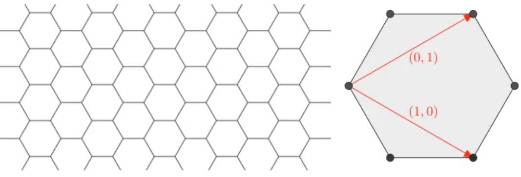
où deux sommets sont reliés, noté x ∼ y, s’il y a une arête entre les deux, c’est-à- dire, s’il existe e ∈ E tel quee = {x, y}. Un homomorphisme α entre deux graphes X = (V, E) et X = (V, E) est donné par deux fonctions V x → αx ∈ V et E e → αe ∈ E tel que si e = {x, y} on a αe = {αx, αy}. On dit que X admet une action de Z^d s’il existe un homomorphisme de groupes entre Z^d et le groupe d’automorphismes de X, noté Aut(X). Souvent on n’écrit pas cet isomorphisme et on dit queZ^d agit surX par automorphismes. En général, pour ce genre de graphes un résultat comme leThéorème 0.1 n’est pas disponible. Cependant, on peut tout de même mentionner [And13] où pour le cas particulier du réseau hexagonal des résultats partiels sont disponibles.

Considérons le graphe infini donné par le pavage hexagonal. Une action deZ²peut être définie comme dans la Figure 0.1. Puisqu’il y a deux orbites des sommets sous l’action deZ², la transformation de Fourier doit être définie à valeurs vectorielles. Plus précisément, siX = (V, E) est le réseau hexagonal, etx₀ety₀sont deux représentants des orbites on peut définir

U :l²(V)→L²(T²;C²) ; (Uf)(ξ) =

μ∈Z²

e^2πiξ^·^μf(μx₀),

μ∈Z²

e^2πiξ^·^μf(μy₀).

(11)

(0,1) (1,0)

Figure 0.1 – Le réseau hexagonal et l’action de Z².

Dans ce cas le Laplacien n’est plus après transformation de Fourier un opérateur de multiplication par une fonction mais plutôt par une matrice. En fait on a :

(UΔU^∗f)(ξ) = −3 1 + e^−2πiξ¹+ e^−2πiξ² 1 + e^2πiξ¹+ e^2πiξ² −3

f₁(ξ) f₂(ξ)

. (3) La forme particulière de cette matrice dépend du choix dex₀ ety₀ mais (3) peut être obtenue en choisissantx₀ et y₀ de sorte qu’ils soient reliés par une arête horizontale.

En calculant les valeur propres de cette matrice on obtient qu’elles sont données par λ_±= 3±3 + 2 cos(2πiξ₁) + 2 cos(2πiξ₂) + 2 cos(2πi(ξ₁−ξ₂)).

Une fois qu’on a trouvé les valeurs on peut répéter l’argument précédent pour l’opéra- teur conjugué sauf que cette fois-ci il a une forme matricielle. En fait, on a le théorème suivant.

Théorème 0.2 ([And13, Theorem 2.7]). Soit X le réseau hexagonal et soit R un potentiel à support compact. Pour H =−Δ +R on a

1. Les valeurs propres deH sont de multiplicité ﬁnie et peuvent s’accumuler seule- ment enτ :={0,2,3,4,6}.

2. H n’a pas de spectre singulier continu.

3. Un principe d’absorption limite est valable en dehors de τ∪σ_p(H).

Le résultat principal de la première partie de cette thèse Theorem 1.2.2 est un résultat similaire aux précédents Théorèmes 0.1 et 0.2 mais qui les généralise dans trois directions. La première est qu’il ne s’adresse pas à un graphe particulier mais à la classe de graphes périodiques connus comme cristaux topologiques suivant les travaux de Sunada [Sun12]. Ces graphes abstractisent la notion d’être invariant par translations pour traiter des graphes qui ne sont pas nécessairement plongés dans un espace Euclidien. Dans ce cas la transformation unitaireU doit être déﬁnie del²(V) dansL²(T^d;Cⁿ), oùnest donné par le nombre d’orbites de sommets sous l’action de Z^d.

Une deuxième direction est de considérer des perturbations du graphe lui-même.

On dit q’un graphe est pondéré s’il est doté d’une mesure mdéﬁnie sur les sommets et sur les arêtes non-orientées. Pour un graphe pondéré (X, m) le Laplacien est donné par

[Δ(X, m)f] (x) =

y∼x

m({x, y})

m(x) (f(y)−f(x)).

(12)

5

On peut donc étudier des perturbations du graphe en imposant qu’une mesure dite perturbée m converge à l’infini vers une mesure périodique m. La périodicité de m est définie par rapport à l’action deZ^d. Pour ce type de perturbations dites métriques un principe d’absorption limite a été démontré dans [AIM16, Theorem 7.7]. Cepen- dant ils considèrent seulement des perturbations compactes, c’est-à-dire quemet m coïncident en dehors d’un ensemble fini de sommets et arêtes.

Finalement une troisième direction est de considérer les potentiels comme dans leThéorème 0.1. Il semble naturel d’ajouter un potentiel périodiqueR₀ à l’opérateur non-perturbé. Ces potentiels deviennent après transformation de Fourier juste un opérateur de multiplication par une matrice diagonale. Il faut noter que dans le cas Z^d ceci revenait juste à ajouter une constante. Donc, comme perturbation on est amené à considérer des potentiels qui tendent à l’inﬁni vers le potentiel périodique R₀. C’est l’action de Z^d qui permet d’étudier cette convergence et de donner une condition du type courte portée. Pour la condition de longue portée on doit trouver l’analogue de la dérivation. On peut voir que la condition naturelle à imposer est une décroissance de

e ={x, y} → |R_l(y)−R_l(x)| (4) où R_l représente la partie à longue portée de la diﬀérenceR−R₀. À nouveau c’est l’action de Z^d, une fois qu’on a choisi des représentants des orbites des arêtes, qui permet de donner des conditions comme celles duThéorème 0.1.

On voudrait maintenant comprendre pourquoi (4) est un condition naturelle. Ceci nous amène à présenter aussi le cadre de la deuxième partie de cette thèse. Pour cela il faut tout d’abord introduire quelques objets. SoitX = (V, E) un graphe. Pour chaque arête non-orientéee={x, y} deE on considère deux arêtes orientées (x, y) et (y, x).

On note par A l’ensemble des arêtes orientées ainsi construites mais on continue de noter pare ces arêtes orientées. On note aussi paro(e) l’origine d’une arête orientée et par t(e) sa cible. De plus, on note par e l’arête opposée à e. Par analogie avec le géométrie différentielle on considère les fonctions définies sur V comme des 0− formes. Donc, les fonctions définies sur les arêtes correspondent à des 1−formes. Plus précisément on définit les espaces de 0−cochaînes C⁰(X) et 1−cochaînesC¹(X) par

C⁰(X) :={f :V →C}; C¹(X) :={f :A→C|f(e) =−f(e)} . On peut maintenant déﬁnir l’analogue discret de la dérivation extérieure par

d:C⁰(X)→C¹(X) ; [df] (e) =f(t(e))−f(o(e)).

On voit donc qu’imposer une décroissance sur (4) correspond bien à imposer une condition sur la dérivée du potentiel. De plus on a bien la factorisationd^∗d= Δ.

Jusqu’à maintenant on a donc considéré des opérateurs différentiels discrets du deuxième ordre perturbés par des opérateurs d’ordre 0. Il semble naturel de se poser la question : est-ce que l’on peut étudier par la méthode à commutateurs des opérateurs différentiels du premier ordre ? La réponse est notreTheorem 2.2.5. Notre opérateur du première ordre est l’opérateur de Gauss-BonnetD introduit dans [AT15]. Puisqu’on veut que formellement D:=d+d^∗ on doit le définir comme suit

D:C⁰(X)⊕C¹(X)→C⁰(X)⊕C¹(X) ; D(f₀, f₁) := 0 d^∗ d 0

f₀ f₁

= (d^∗f₁, df₀).

(13)

Pour étudier cet opérateur la transformation unitaireU doit s’étendre àl²(X) = l²(V)⊕l²(E) à valeur dans L²(T^d;C^n+l), où l est donné par le nombre d’orbites d’arêtes sous l’action deZ^d. Pour cet opérateur il n’y avait pas de résultats disponibles pour des graphes périodiques généraux mais on peut tout de même faire référence à [GH14]. Dans cette référence, l’opérateur dit de Dirac discret est étudié surl²(Z;C²).

Il est déﬁni pourm≥0 par

−D_m:= −m (S₁−1) (S₁^∗−1) m

.

Dans ce cas, la structure de graphe est cachée derrière le fait qu’il y a une corres- pondance bijective entre les arêtes non orientées et Z. Cette identiﬁcation donne l’équivalence entred et S₁−1. Leur résultat est le suivant.

Théorème 0.3 ([GH14, Theorem 1.2]). SoitR∈l^∞(Z;R²) etα∈Navec

n→±∞lim R(n) = 0 (5)

R_|_Z

+−S₁^αR_|_Z

+ ∈l¹(Z+,R²) . (6)

Alors le spectre de l’opérateur perturbéH :=D_m+Rest purement absolument continu dans(−√

m²+ 4,−m)∪(m,√

m²+ 4).

Dans le Theorem 2.2.5 nos conditions sont à nouveau données en termes de dé- croissance pour le potentiel qui maintenant doit être déﬁni sur les sommets et sur les arêtes. De plus nous traitons, comme pour le Laplacien, des perturbations de courte portée de la métrique.

Un autre type de problèmes est d’étudier les analogues discrets des opérateurs magnétiques. Le Laplacien magnétique pour un graphe généralX = (V, E) est déﬁni à partir d’un potentiel magnétique ϕ : V ×V → R tel que ϕ(x, y) = −ϕ(y, x). On peut alors déﬁnir Δϕ dans l²(V) par

[Δ_ϕf] (x) =

y∼x

e^iϕ(x,y)m({x, y})

m(x) (f(y)−f(x)).

L’idée d’un analogue discret des opérateurs magnétiques a ses racines dans le modèle de Harper. Ce modèle a reçu beaucoup d’attention à cause de ses propriétés spectrales particulières. L’opérateur de Harper est un opérateur de Schrödinger magnétique sur Z² avec un champ magnétique constant. Il peut être défini en choisissant deux constantes α₁ et α₂ tel que α₂−α₁ =: θ correspond, dans le cas continu, au flux du champ magnétique à travers une cellule unité. Si on note par {δ_j}j=1,2 la base canonique deZ², le potentiel magnétique est défini par

ϕ(μ, γ) =

⎧⎪

⎪⎪

⎪⎨

⎪⎪

⎩

−α₁μ₂ siγ−μ=δ₁ α₁μ₂ siγ−μ=−δ₁

−α₂μ₁ siγ−μ=δ₂ α₂μ₁ siγ−μ=−δ₂

(7)

(14)

7

et on déﬁnit l’opérateur de multiplication R par R(μ) = 2(cos(α₁μ₂) + cos(α₂μ₁)).

Donc, pour ces fonctionϕet Ret des poids triviaux, l’opérateur de Harper est déﬁni parH_α₁_,α₂ = Δϕ+R. En eﬀet on a :

[Hα₁,α₂f] (μ) = e⁻îα¹^μ²f(μ+δ₁)+eîα¹^μ²f(μ−δ₁)+e⁻îα²^μ¹f(μ+δ₂)+eîα²^μ¹f(μ−δ₂). En contraste avec le cas continu, le spectre deH_α₁_,α₂ dépend fortement du paramètre θ. Parmi les différentes approches utilisées pour étudier ce problème, lesC^∗−algèbres sont un outil puissant qui permet d’étudier l’opérateur de Harper mais aussi ses généralisations. Ceci est motivé par la remarque suivante. Définissons deux opérateurs unitaires dansl²(Z²)U et V par

U : =e⁻^iα²^N¹S₂ V : =e⁻^iα¹^N²S₁ . Donc on a

H_α₁_,α₂ =V +V^∗+U+U^∗ . (8) L’importance de (8) est qu’il montre que H_α₁_,α₂ est dans laC^∗-algèbre engendrée par U et V. Puisque U et V satisfont

U V = e^iθU V (9)

cette algèbre correspond à une représentation dans l²(Z²) de l’algèbre des rotations Aθ. Ceci explique pourquoi H_α₁_,α₂ présente des propriétés spectrales diﬀérentes si θ ∈Q ouθ /∈Q. Par exemple, siθ ∈Q, on peut montrer queH_α₁_,α₂ a une structure de bandes [Sun94] tandis que siθ /∈ Qle spectre est un ensemble de Cantor [AJ09].

D’un autre côté, le fait que{Aθ}θ∈[0,2π] soit un champ continu deC^∗−algèbres a été exploité pour montrer que les bords du spectre deH_α₁_,α₂ sont continus quand on fait varierθ:=α₂−α₁. En eﬀet, la continuité Lipschitz ou Hölder peut être montrée dans certains cas.

Dans la troisième partie de cette thèse nous nous intéressons au problème de la continuité du spectre pour des opérateurs de Schrödinger magnétiques agissant sur l²(Z^d). Ils sont déﬁnis par un symbolehet un potentiel magnétiqueϕet agissent par

[Hf] (μ) :=

γ∈Z^d

h(μ;γ−μ)e^iϕ(μ,γ)f(γ). (10)

Sous certaines conditions surh, (10) déﬁnit un opérateur borné auto-adjoint. De plus pour leϕdéﬁni par (7) et

h(μ;γ) =

1 si|γ|= 1

0 si non, (11)

l’opérateur de Schrödinger magnétique H déﬁni par (10) coïncide avec H_α₁_,α₂. De tels opérateurs ont été étudiés dans [Nen05] sous le nom d’opérateurs de Harper généralisés. Sous une condition de décroissance exponentielle de h, il est montré que les bords du spectre d’une famille d’opérateurs H varie, à un facteur près, de façon Lipschitz quand on fait varier un potentiel ﬁxé de façon multiplicative :i.e. ϕ=ϕ.

(15)

Notre approche est tout autre parce qu’on cherche sous quelle hypothèse on peut faire varier et le symbolehet le potentielϕde manière à assurer la continuité des composantes spectrales. Cette approche suit la tradition de l’utilisation desC^∗−algèbres car notre premier pas est de trouver uneC^∗−algèbre et une représentation de cette algèbre dans l²(Z^d) telle que les opérateurs de Schrödinger magnétiques soient dans l’image. Ce prérequis correspond à l’analogue de (8). Dans ce cadre, l’aspect magné- tique est encodé par la représentation et donc pour chaque élément de laC^∗−algèbre on a un opérateur magnétique correspondant. Le résultat principal de cette partie est leTheorem 3.3.3où sous des hypothèses de continuité d’une famille d’éléments de la C^∗−algèbre on obtient la continuité des composantes spectrales de ses représentations magnétiques. Ce résultat abstrait permet à son tour de montrer leTheorem 3.1.2qui correspond au cas traité dans de la référence [Nen05].

On termine cette introduction en présentant la structure de cette thèse. LeCha- pitre 1traite du problème des opérateurs de Schrödinger sur des cristaux topologiques.

Ce chapitre correspond à la prépublication

— D. Parra, et S. Richard, Spectral and Scattering theory for Schrödinger ope- rators on perturbed topological crystals, arXiv:1607.03573.

Le Chapitre 2 utilise en partie les résultats abstraits du Chapitre 1 pour étudier d’autres types d’opérateurs déﬁnis sur des cristaux topologiques. Il correspond à la prépublication

— D. Parra,Spectral and Scattering theory for Gauss-Bonnet operators on per- turbed topological crystals, arXiv:1609.02260.

Finalement, le Chapitre 3 présente des résultats de continuité du spectre pour des familles d’opérateurs de Schrödinger magnétiques et correspond à l’article publié

— D. Parra, et S. Richard, Continuity of the spectra for families of magnetic operators on Z^d, Anal. Math. Phys.6 no. 4, 327–343, 2016.

(16)

Chapter 1 Schrödinger operators

1.1 Introduction

The aim of this chapter is to describe the spectral theory of a Schrödinger opera- torH acting on a perturbed periodic discrete graph. The main strategy is to exploit the fibered decomposition of the periodic underlying operatorH₀in the unperturbed graph to get a Mourre estimate. Then, by applying perturbative techniques, the description of the nature of the spectrum ofH can be deduced: it consists of absolutely continuous spectrum, of a finite number (possibly zero) of eigenvalues of infinite multiplicity, and of eigenvalues of finite multiplicity which can accumulate only at a finite set of thresholds. The scattering theory for the pair (H, H₀) is also investigated.

The study of Laplace operators on infinite graphs has recently attracted lots of attention. Let us mention for example the problem of essential self-adjointness for very general infinite graphs [GS11; Kel15], or the more precise study of the spectrum for bounded Laplacians [AH09; MRT07]. For periodic graphs it is well-known that this spectrum has a band structure with at most a finite number of eigenvalues of infinite multiplicity [HN09]. This structure is preserved if one considers periodic Schrödinger operators [KS14;KS15b;KS15a]. Our interest is in what happens when such periodic Schrödinger operators are perturbed.

The perturbations we consider are of two types. On the one hand we add a potential that decays at inﬁnity either as a short-range or as a long-range function.

To the best of our knowledge this has not been studied for general periodic graphs and only the case of Z^d has been fully investigated in [BS99]. In that respect, our main theorem generalizes such results to arbitrary periodic graphs. Note that some related results on the inverse scattering problem are available forZ^din [IK12] and the hexagon lattice in [And13], but only compactly supported perturbations are considered.

The second types of perturbations we consider correspond to the modiﬁcation of the graph itself. This kind of perturbations has recently been studied in [SS15] for investigating the stability of the essential spectrum. In [AIM16] results similar to ours are exhibited, but the perturbations considered there are only compactly supported and some implicit conditions on the Floquet-Bloch variety are assumed. These two restrictions do not appear in our work. Let us still mention the related work [CT13]

where compactly supported perturbation are considered in the framework of a regular tree.

9

(17)

As pointed before, the two main tools that we use is the Floquet-Bloch decomposition of periodic Schrödinger operator and Mourre theory. This decomposition is an important tool for the analysis of the periodic graphs and we mention only a few arti- cles that use it [And13;AIM16; HN09;KS14;KSS98]. For Mourre theory, we refer to [ABG96] for the general theory and to [GN98b] for this theory applied to analytically ﬁbered operators from which our work is inspired. In the discrete setting, this theory has already been used for example in [AF00; MRT07]. In the special case of the graph Z^d, it plays a central role in [BS99]. Mourre theory for more general periodic graphs has also been mentioned in [HN09] for proving that the Laplace operator has a purely absolutely continuous spectrum outside some discrete spectrum. However, since no perturbation were considered in that paper, the theory was not further developed.

Our work can thus also be seen as an extension of that work.

Finally, we would like to stress that several deﬁnitions of periodic graphs can be found in the literature. We have opted for the setting of topological crystals which has the advantage that no embedding in the Euclidean space is needed. We refer to [Sun12] for a thorough introduction to topological crystals and to many examples of such structures.

Let us still mention that in this chapter we restrict our attention to Laplace operators acting on the vertices of the graph. InChapter 2, Gauss-Bonnet operators are studied, as well as the Laplacian acting on edges [BGJ15]. Note that the Gauss- Bonnet operator is a Dirac-type operator that acts both on vertices and edges. This operator has recently been investigated in [AT15; GH14].

We finally describe the content of this chapter. In Section 1.2 we describe the framework of our investigations and provide our main result. Under suitable assumptions it consists in the description of the spectral type of the operators under inves- tigation, and in the existence of suitable wave operators. More precise information on the purely periodic setting are then presented in Section 1.3 and we show that the periodic operator H₀ can be decomposed into a family of magnetic Schrödinger operators. InSection 1.4 it is proved that the latter operator is unitarily equivalent to an analytically fibered operator. In order to be self-contained, a brief review on real analyticity and a few definitions and results are provided. Section 1.5 is dedi- cated to the conjugate operator theory, also called Mourre theory. For completeness, we first describe the abstract framework of this theory, and provide then a thorough construction of the necessary conjugate operator. In fact, this construction is inspired from [GN98b] but part of the argumentation has been simplified for our context. In addition, we can take advantage of the recent reference [RT09] which supplies a lot of information on toroidal pseudodifferential operators. Based on all these preliminary constructions, the proof of the main theorem is given in Section 1.6. A first preliminary subsection discuses the regularity of some abstract operators with respect to the newly constructed conjugate operator, and these results are finally applied to operators appearing in our context of the perturbation of a periodic graph.

1.2 Framework and main result

In this section we describe the framework of our investigations and state our main result.

(18)

1.2. FRAMEWORK AND MAIN RESULT 11 A graph X =V(X), E(X)is composed of a set of vertices V(X) and a set of unoriented edgesE(X). Graphs with loops and parallel edges are accepted. Generi- cally we shall use the notationx, y for elements ofV(X), and e ={x, y}for elements ofE(x). If bothV(X) andE(X) are ﬁnite sets, the graph X is said to be ﬁnite.

A morphismω :X →Xbetween two graphs X andX is composed of two maps ω : V(X) → V(X) and ω : E(X) → E(X) such that it preserves the adjacency relations between vertices and edges, namelyω(e) ={ω(x), ω(y)}. Let us stress that we use the same notation for the two mapsω:V(X)→V(X) andω:E(X)→E(X), and that this should not lead to any confusion. An isomorphism is a morphism that is a bijection on the vertices and on the edges. The group of isomorphisms of a graph X into itself is denoted by Aut(X). For a vertex x ∈ V(X) we also set E(X)x:={e∈E(X)|x∈e}. If E(X)x is ﬁnite for everyx ∈V(X) we say that X is locally ﬁnite.

A morphismω:X →Xbetween two graphs is said to bea covering map if (i) ω:V(X)→V(X) is surjective,

(ii) for all x∈V(X), the restrictionω|_E(X)_x:E(X)x →E(X)_ω(x)is a bijection.

In that case we say that X is a covering graph over the base graph X. For such a covering, we deﬁne the transformation group of the covering as the subgroup of Aut(X), denoted by Γ, such that for every μ∈Γ the equality ω◦μ=ω holds. We now deﬁne a topological crystal, and refer to [Sun12, Sec. 6.2] for more details.

Deﬁnition 1.2.1. A d-dimensional topological crystal is a quadruplet (X,X, ω,Γ) such that:

(i) X is an inﬁnite graph, (ii) Xis a ﬁnite graph,

(iii) ω:X →X is a covering map,

(iv) The transformation group Γ of ω is isomorphic to Z^d,

(v) ω is regular, i.e. for every x, y ∈ V(X) satisfying ω(x) = ω(y) there exists μ∈Γ such that x=μy.

We will usually say that X is a topological crystal if it admits a d-dimensional topological crystal structure (X,X, ω,Γ). Note that all topological crystal are locally ﬁnite, with an upper bound for the number of elements in E(X)x independent ofx.

Indeed, the local finiteness and the fixed upper bound follow from the definition of a covering and the assumption (ii) of the previous definition.

From the set of unoriented edges E(X) of an arbitrary graph X we construct the set of oriented edges A(X) by considering for every unoriented edge{x, y} both (x, y) and (y, x) in A(X). The elements of A(X) are still denoted by e. The origin vertex of such an oriented edge e is denoted by o(e), the terminal one byt(e), and e denotes the edge obtained from e by interchanging the vertices, i.e. o(e) =t(e) and t(e) =o(e). For x ∈ V(X) we set A(X)x ≡A_x := {e ∈A(X) | o(e) =x}. Clearly, any morphismω between a graph X and a graph X, and in particular any covering map, can be extended to a map sending oriented edges ofA(X) to oriented edges of A(X). For this extension we keep the convenient notationω:A(X)→A(X).

Ameasure mon a graphX is a strictly positive function deﬁned on vertices and on unoriented edges. On oriented edges, the measure satisﬁes m(e) = m(e). From

(19)

now on, let us assume that the graphX is locally ﬁnite. For such a graph the Laplace operator is deﬁned on the space of 0-cochains C⁰(X) :={f |V(X)→C} by

[Δ(X, m)f] (x) =

e∈Ax

m(e) m(x)

ft(e)−f(x), ∀f ∈C⁰(X).

Furthermore, when

deg_m:V(X)→R+, deg_m(x) :=

e∈Ax

m(e)

m(x) (1.1)

is bounded, the operator Δ(X, m) is a bounded self-adjoint operator in the Hilbert space

l²(X, m) =f ∈C⁰(X)| f²:=

x∈V(X)

m(x)|f(x)|²<∞ endowed with the scalar product

f, g=

x∈V(X)

m(x)f(x)g(x) ∀f, g∈l²(X, m).

Let us now consider a topological crystal X, a Γ-periodic measure m₀ and a Γ- periodic functionR₀ :V(X) →R. The periodicity means that for every μ∈Γ,x ∈ V(X) and e∈E(X) we havem₀(μx) =m₀(x),m₀(μe) =m₀(e) andR₀(μx) =R₀(x).

We can then provide the deﬁnition of a periodic Schrödinger operator. It consists in the operator

H₀ :=−Δ(X, m0) +R₀. (1.2) Note that we use the same notation for the function R₀ and for the corresponding multiplication operator. As a consequence of our assumptions, the expression H₀ deﬁnes a bounded self-adjoint operator in the Hilbert spacel²(X, m₀).

Our aim is to study rather general perturbations of the operator H₀. In fact, we shall consider two types of perturbations. The ﬁrst one consists in replacing the multiplication operator by a function R which converges rapidly enough to R₀ at inﬁnity. The precise formulation will be provided in the subsequent statement. The other type of perturbation is more substantial and consists in modifying the measure on the graph. For that purpose, we shall consider a second strictly positive measure monX, and which converges in a suitable sense to the Γ-periodic measure m₀. The corresponding perturbed operator acts then in the Hilbert spacel²(X, m) and has the form

H =−Δ(X, m) +R. (1.3) Let us stress that this modification of the measure naturally leads to a two- Hilbert space problem since the measures m₀ and m enter into the definition of the underlying Hilbert spaces. Fortunately, since the graph structure is not modified, a unitary transformation between both spaces is at hand. Namely, we consider J : l²(X, m)→l²(X, m₀) defined by

[Jf](x) =

m(x) m₀(x)

¹₂

f(x), f ∈l²(X, m). (1.4)

(20)

1.2. FRAMEWORK AND MAIN RESULT 13 Note that this map is well-deﬁned and unitary since m₀(x) and m(x) are assumed to be strictly positive for any x∈V(X). The inverse of J is given by [J^∗f](x) = _m₀_(x)

m(x)

¹₂

f(x). The fact that J is unitary plays an essential role in the comparison of both operators.

We have now almost all the ingredients for stating our main result. The missing ingredient is the deﬁnition of the entire part of a vertex and of an edge, denoted respectively by [x] ∈ Γ and [e] ∈ Γ, see (1.8) and (1.9) for the details. Indeed, in order to properly introduce these notions some additional deﬁnitions are necessary and we have decided to postpone them to the next section. We still mention that the isomorphism between Γ andZ^d allows us to borrow the Euclidean norm| · |ofZ^d and to endow Γ with it. As a consequence of this construction, the notations|[x]|and|[e]|

are well-deﬁned, and the notion of rate of convergence towards inﬁnity is available.

Theorem 1.2.2. Let X be a topological crystal. Let H₀ and H be deﬁned by (1.2) and (1.3) respectively. Assume that msatisﬁes

_∞

1

dλ sup

λ<|[e]|<2λ

m(e)

m(o(e))− m₀(e) m₀(o(e))

<∞ . (1.5)

Assume also that the diﬀerence R−R₀ is equal to R_s+R_l which satisfy _∞

1

dλ sup

λ<|[x]|<2λ|R_s(x)|<∞, (1.6) and

R_l(x)−−−→^x→∞ 0, and

_∞

1 dλ sup

λ<|[e]|<2λ

R_lt(e)−R_lo(e)<∞ . (1.7)

Then, there exists a discrete set τ ⊂ R such that for every closed interval I ⊂ R\τ the following assertions hold:

1. H₀ has not eigenvalues inI and H has at most a ﬁnite number of eigenvalues inI and each of these eigenvalues is of ﬁnite multiplicity,

2. σ_sc(H₀)∩I =σ_sc(H)∩I =∅, 3. If R_l≡0, the local wave operators

W_±≡W_±(H, H₀;J^∗, I) =s− lim

t→±∞e^iHtJ^∗e^−iH⁰^tE_H₀(I)

exist and are complete, i.e. Ran(W₋) = Ran(W+) = E_H^ac(I)l²(X, m). Since σ_sc(H) =∅ they are indeed asymptotically complete.

Note that the operator J^∗ enters into the deﬁnition of the wave operators (in- stead of the more traditional notationJ) since we have deﬁnedJ froml²(X, m) to l²(X, m₀). This choice is slightly more natural in our context.

The hypothesis (1.5) and (1.6) are usually referred to as a short-range type of decay. In particular it is satisﬁed for functions that decay faster thanC(1 +|[x]|)⁻¹⁻

for some constantCindependent ofx. It is worth mentioning that that condition (1.5) is quite general and is automatically satisfied if the differencem−m₀ itself satisfies a short-range type of decay. For example if we assume that|m(e)−m₀(e)| ≤ C(1 +

(21)

|[e]|)⁻¹⁻and|m(x)−m₀(x)| ≤C(1 +|[x]|)⁻¹⁻, then (1.5) is satisﬁed. On the other hand (1.7) is usually called along-rangedecay since the diﬀerence R_lt(e)−R_lo(e) should be thought as the derivative ofR_lat the point o(e) in the direction e. To sum up we can say that we cover perturbations by short-range and long-range potentials but only by short-range perturbation of the metric.

Remark 1.2.3. A more drastic modification would be to allow m(x) = 0 for some x∈V(X), and this would roughly correspond to the suppression of some vertices in the graph. Reciprocally, it would also be natural to consider a perturbation of the operator H₀ on the topological crystalX by the addition of some vertices toX. Note that these modifications are more difficult to encode since there would be no natural unitary operator available between the corresponding Hilbert spaces. These perturbations will not be considered in the present but we intend to come back to them in the future.

1.3 Periodic operator and its direct integral decomposition

The aim of this section is to provide some additional information on the periodic Schrödinger operator and to show that this operator can be decomposed into the direct integral of magnetic Schrödinger operators deﬁned on the small graphX. This decomposition is an important tool for studying its spectral properties, as shown for example in [And13; HN09; KS14; KSS98].

Let us consider a topological crystal (X,X, ω,Γ). The notation x, resp. x, will be used for the elements of V(X), resp. of V(X), and accordingly the notation e, resp. e, will be used for the elements of E(X), resp. of E(X). It follows from the assumption (v) inDeﬁnition 1.2.1thatX\Γ∼=X, and therefore we can identifyV(X) as a subset of V(X) by choosing a representative of each orbit. Namely, since by assumption V(X) = {x1, . . . ,xn} for some n ∈ N, we choose {x₁, . . . , x_n} ⊂ V(X) such that ω(xj) = xj for any j ∈ {1, . . . , n}. For shortness we also use the notation ˇ

x := ω(x) ∈ V(X) for any x ∈ V(X), and reciprocally for any x ∈ X we write ˆx∈ {x₁, . . . , x_n}for the unique elementx_j in this set such that ω(xj) =x.

As a consequence of the previous identification we can also identify A(X) as a subset of A(X). More precisely, we identify A(X) with ∪ⁿ_j=1A_x_j ⊂ A(X) and use notations similar to the previous ones: For any e∈A(X) one sets ˇe =ω(e)∈A(X), and for any e∈ A(X) one sets ê ∈ ∪ⁿ_j=1A_x_j for the unique element in this set such thatω(ê) = e. Let us stress that these identifications and notations depend only on the initial choice of{x₁, . . . , x_n} ⊂V(X).

We have now enough notations for deﬁning the entire part of a vertex x as the map [·] :V(X)→Γ satisfying

[x]xˇ=x . (1.8)

Similarly, the entire part of an edge is deﬁned as the map [·] :A(X)→Γ satisfying

[e]ˇe = e . (1.9)

The existence of this function [·] follows from the assumption (v) ofDeﬁnition 1.2.1 on the regularity of a topological crystal. One easy consequence of the previous construction is that the equality [e] = [o(e)] holds for any e∈A(X).