A family of simple paternalistic transfer models - Repository of the Academy's Library

MŰHELYTANULMÁNYOK DISCUSSION PAPERS

INSTITUTE OF ECONOMICS, CENTRE FOR ECONOMIC AND REGIONAL STUDIES, HUNGARIAN ACADEMY OF SCIENCES BUDAPEST, 2013

MT-DP – 2013/24

A family of simple paternalistic transfer models

ANDRÁS SIMONOVITS

Discussion papers MT-DP – 2013/24

Institute of Economics, Centre for Economic and Regional Studies, Hungarian Academy of Sciences

KTI/IE Discussion Papers are circulated to promote discussion and provoque comments.

Any references to discussion papers should clearly state that the paper is preliminary.

Materials published in this series may subject to further publication.

A family of simple paternalistic transfer models Author:

András Simonovits research advisor Institute of Economics

Centre for Economic and Regional Studies Hungarian Academy of Sciences

also Mathematical Institute, Budapest University of Technology, and Department of Economics, CEU

email:[email protected]

August 2013

ISBN 978-615-5243-81-3 ISSN 1785 377X

A family of simple paternalistic transfer models András Simonovits

Abstract

A general framework is analyzed which contains several special transfer (tax and pension) models. In our static two-overlapping-generation framework, every individual works in the first stage of the adult age, while is retired in the second. The government operates a balanced linear transfer system, sometimes with caps. In the models, the individuals may optimize their situation in various ways: contributing to voluntary pension, restraining labor supply and underreporting wages. Individuals are typically short-sighted, therefore they choose paternalistically suboptimal decisions. The models provide useful information on the socially optimal paternalistic transfer system.

Keywords: tax systems, pension systems, pension models, overlapping generations, paternalism

JEL classification: H24, I31, J22, J26 Acknowledgements:

I am indebted to the support of the Hungarian Science Research Foundation's project K 67853. I express my general gratitude to the help of those who helped me writing the papers underlying the present paper. Erzsébet Kovács and Balázs Muraközy's useful comments are also acknowledged.

Egyszerű paternalista transzfermodellek családja Simonovits András

Összefoglaló

Olyan általános keretet elemzünk, amely néhány speciális transzfer (adó- és nyugdíj-) modellt tartalmaz. Statikus, két együtt élő nemzedékes keretünkben minden egyén dolgozik az első időszakban, és nyugalomban van a másodikban. A kormányzat kiegyensúlyozott lineáris transzferrendszert működtet, néha plafonokkal. Modelljeinkben az egyének helyzetüket különféleképp optimalizálhatják: részt vesznek egy önkéntes nyugdíjrendszerben, visszafogják munkakínálatuk és eltitkolják keresetük egy részét. Az egyének rendszerint rövidlátók, ezért paternalista szempontból szuboptimális döntéseket hoznak. A modellek hasznos információkat adnak a társadalmilag optimális paternalista transzferrendszerekről.

Tárgyszavak: adórendszerek, nyugdíjrendszerek, nyugdíjmodellek, együtt élő nemzedékek, paternalizmus

JEL kód: H24, I31, J22, J26

family2 quadratic

A family of simple paternalistic transfer models

by

Andr´as Simonovits

Institute of Economics, CERS, Hungarian Academy of Sciences also Mathematical Institute, Budapest University of Technology,

and Department of Economics, CEU Budapest, Buda¨orsi ´ut 45, Hungary

[email protected] July 20, 2013

Abstract

A general framework is analyzed which contains several special transfer (tax and pen- sion) models. In our static two-overlapping-generation framework, every individual works in the first stage of the adult age, while is retired in the second. The govern- ment operates a balanced linear transfer system, sometimes with caps. In the models, the individuals may optimize their situation in various ways: contributing to voluntary pension, restraining labor supply and underreporting wages. Individuals are typically short-sighted, therefore they choose paternalistically suboptimal decisions. The models provide useful information on the socially optimal paternalistic transfer system.

Keywords: tax systems, pension systems, pension models, overlapping generations, paternalism

JEL numbers: H24, I31, J22, J26

∗ I am indebted to the support of the Hungarian Science Research Foundation’s project K 67853.

I express my general gratitude to the help of those who helped me writing the papers underlying the present paper. Erzs´ebet Kov´acs and Bal´azs Murak¨ozy’s useful comments are also acknowledged.

1. Introduction

I have recently analyzed several simple transfer (i.e. tax-and-pension) models (some- times written with coauthors) almost independently of each other. Simple means here utmost simplicity: everything is neglected what can be neglected. Having completed their analyses, the joint features of the models became much clearer. (i) Though they follow the logic of the Overlapping Generations model (cf. Weil, 2008), they are basi- cally static, i.e. they only consider a population consisting of people born in the same time period (year). (ii) They assume away the changes in wages and pensions occurring during the two life stages. (iii) The population is heterogeneous, the types’ earnings or discount factors are different. (iv) The rules of the transfer system strongly influence individual behavior, based on maximization of discounted utility: labor supply, saving at young age, report on earnings etc. (v) The paternalistic government determines the transfer rules by maximizing an undiscounted social welfare function.¹

Of course, these models were not the first ones of this type. Nevertheless, I give a sur- vey of them. For reference points, I single out three such models which preceded mines:

Feldstein (1985), (1987) (twins) and Cremer, De Donder, Maldonaldo and Pestieau (2008).² I only mention few related but complex models which have dynamic and detailed age-structures: Auerbach and Kotlikoff (1987), Fehr and Habermann (2008), Sefton, van de Ven and Weale (2008).³ It is of interest that the complex models gener- ally neglect myopia (for an exception, Fehr and Kindermann, 2010). Note that all these models overlooked the complex formulation of mechanism design invented by Mirrlees (1971) and treated in an introductory way by Diamond (2003) in a two-generation framework.

Table 1 surveys the types of assumptions of the foregoing models. The order of discussion follows the order of complexity. For the sake of clarity, I will refer to my models and the underlying assumptions by keywords. To avoid any confusion, however, I give here their resolutions.

I start with the models’ abbreviations. Voluntary pension: Simonovits (2009a) and (2011b), cap on contributions: Simonovits (2012a) and (2013), labor supply: Simonovits (2012d), wage reporting: Simonovits (2009b), pension credit: Simonovits (2012c). Con- tinuing with the assumptions; labor supply: labor supply is flexible; wage report: the reported earnings are endogenous; saving: there exist positive private life-cycle savings (with or without tax favors), nonlinearity: mostly piecewise linearity; tax: in addition to pension contribution, there is a personal income tax. Sign + stands for a property present or endogenous; sign – stands for a property missing or exogenous. (In contrast to some authors, negative savings are excluded!)

1 For the prosand cons of paternalism, see e.g. Sunstein and Thaler (2003) and Epstein (2007), respectively.

2 Cremer and Pestieau (2011) surveyed the whole field.

3 Andersen (2012) is an interesting crossover being a simple dynamic model, investigating the question of more saving or later retirement is better against population aging. Varian (1980) is a simple static model covering the issue of social insurance.

Table 1. Models and assumptions

Assumptions Labor Wage Nonlin-

supply report Saving earity Tax

Models

Feldstein – – + + –

Cremer et al. + – + – –

Voluntary pension – – + + +

Cap on contribution – – + + –

Labor supply + – – – +

Report – + + – –

Pension credit + – + + –

At surveying the results, I pay little attention to the specific issues, rather I con- centrate on the similarities. Nevertheless, it is worth summarizing in a nutshell the messages of the specific models and sometimes illustrating their weights by Hungarian or international data.

a) The voluntary pension system complements or supplements a mandatory one.

Taking into account the arising tax expenditures, the voluntary system is not as attrac- tive as is frequently depicted. Among others, Engen, Gale and Scholz (1996); Baily and Kirkegard (2009, 452–461) emphasize the illusory effects of savings incentives.⁴

b) The cap on the pension contribution base is quite neglected in the literature.

Barr and Diamond (2008, p. 63) list two functions: (i) In a proportional system, the government has no mandate to force high old-age consumption on high-earners. (ii) In a progressive system, the cap limits the redistribution from the rich to the poor. Others discuss a third function: to limit the perverse redistribution from the poor to the rich caused by the strong correlation between lifetime earning and life expectancy. We add a fourth one: the cap reduces the effective contribution rate of those who earn above the cap and thus making room for the presumably more efficient private savings.⁵

c) Designing an optimal transfer system, the elasticity of labor supply plays a key role. First, it limits the scope of redistribution; second, at least in our model, ensuring old-age living standard has a priority over the earning redistribution. (Disney (2004) thoroughly analyzes the redistribution in various public pension systems.) Nevertheless, the impact of elasticity of labor supply is a hotly debated issue. We only mention that the Czech Republic, which is quite similar to Hungary in many respects, is able to operate a strongly redistributive pension system without having significant other pillars (see also underreported earnings below).

4 For example, in Hungary, in 2009 the voluntary contributions—mostly paid by the well-to-do—

amounted only to 0.3 percent of the GDP but requested a 50 percent matching rate. (For comparison, the mandatory pension expenditures were about 10 percent of the GDP in 2009.)

5 The example of Hungary is illuminating: Between 1992 and 2012 the relative value of the cap oscillated between a high 3 and a low 1.6. Since 2013, there is no cap and the benefit has become unlimited as well, creating unwanted tensions and reducing the long-run welfare around 0.7 percent in our model.

d) In the wage reporting model, the unobservable tax morale explains the variation of reported income regardless of the tax rate and the probability of audits and fees (Frey and Weck-Hannemann, 1984).⁶ Our discussion extends the validity of the tax model (e.g. Simonovits, 2011a) to the pension system.⁷ The basic insight is intuitive: the higher the tax morale, the more redistributive the socially optimal transfer system.

e) Rather than choosing between two rigid schemes, namely the flat and the means- tested ones, a lot of countries have been applying the pension credit system. Sefton et al. model the corresponding British system. For example, raising the value of the basic benefits and withdrawing 50 percent of the proportional benefits from the basic pension, the poorest pensioners’ standard of living could be increased without burdening the budget with a uniform basic pension.

Finally we must mention the missing topic of mandatory private pension systems.

For a number of works (e.g. World Bank, 1994), this is the most important issue of the pension reforms. Though the early work of Barr (1979) had already exposed the theo- retical flaws of this approach, only the recent international financial crisis demonstrated the practical problems of such a system and of the transition leading to it.⁸

Having listed these models, a natural question arises: Why do I not unify all these simple models into one? My answer is as follows: The unification would only complicate the model without bringing us too much closer to the reality; dynamics would still be missing, the age-dependence of earnings and of pensions would still be neglected.

The negation of dynamics is especially hurting: a) the contradiction between popula- tion aging and productivity rise is left out; b) the adverse impact of erratically changing government policies (e.g. in Hungary as well as in Great Britain) on the incentive schemes is overlooked; and c) it is impossible to model the transition from one system into another within our two-generation framework. Finally we allude to an alternative of the welfare approach, namely the political economy (cf. Casamatta, Cremer and Pestieau, 2000).

The structure of the remaining part is as follows: Section 2 analyzes three intro- ductory examples: (i) the limits on redistribution with flexible labor supply without old-age consumption; (ii) the relation of the insufficient private saving and the manda- tory pension system of a representative agent; (iii) the practical impossibility of full intra- and intergenerational redistribution. Section 3 presents the general framework.

Section 4 outlines the specific pension models mentioned above. Section 5 returns to the basic specifications in the original papers: discounted Leontief utility function and the continuous Pareto earnings distribution, applied to the calculation of the optimal contribution rate and of the cap; and the pension credit. (An additional gain is that comparing Sections 4 and 5 underlines the excessive sensitivity of our results to appar- ently unessential details.) Section 6 draws the conclusions. At the end of the paper a list contains the notations.

6 An alternative approach is the elasticity of taxable income, for the latest survey, see Saez, Slemrod and Giertz (2012).

7 As a detour, let us call the reader’s attention to two related works: Garay, Simonovits and T´oth (2011) analyzed the dynamics of tax declaration with the traditional methods, while M´eder, Simonovits and Vincze (2012) did the same with the new tools of agent-based modeling.

8 As an afterthought, I mention van Groezen, Leers and Meijdam (2003) whose static protomodel considers the problem of optimal saving and fertility in a similar framework.

2. Introductory examples

As an introduction into models of the transfer systems, we consider the three simplest paternalistic models: one for income redistribution, another for pension and a third for their unification.

2.1. Income redistribution with flexible labor supply

We consider a static model (cf. Simonovits, 2012b) for income redistribution with more than one type. To make the model as simple as possible, we confine our attention to the personal income tax and neglect any other tax or pension. Letw be the total wage (or full compensation) rate of a certain type of workers, T be his annual (or life) time limit, l be his corresponding labor supply, 0 < l < T, then wl is his earning. Let θ be the personal income tax rate (representing all other taxes as well), 0≤θ ≤1 and γ be the basic income. His consumption is equal to

c=γ+ (1−θ)wl.

We turn to the determination of the optimal labor supply. The simplest utility function is copied from Doerrenberg, Duncan, Fuest and Peichl (2012):

U(w, c, l) =c+ 1 2wl².

Substituting the formula of the consumption into the utility function, we arrive at the reducedutility function with parameter w and variable l:

U^∗(w, l) =γ+ (1−θ)wl− 1 2wl².

Take the value of the basic income as given. Due to the strict concavity of U^∗, the optimal labor supply is determined as a root of the marginal utility–labor supply function:

0 =U_l^∗0(w, l) = (1−θ)w−wl.

We have arrived to

Lemma 1. The optimal labor supply and the utility function are equal to l^∗ = 1−θ and U^∗(w, l^∗) =γ + 1

2w(1−θ)².

Ceteris paribus, the optimal labor supply is independent of the wage rate and of the basic income and is a decreasing function of the tax rate.

Having determined the individual optima, we turn to the macrorelations. Denoting expectation over the wage distribution by E, and choosing an appropriate unit of mea- surement, the average wage rate can be taken unity: E(w) = 1. Then the tax balance is given by

γ =θE(wl^∗) =θ(1−θ).

To determine the socially optimal tax system, we shall use the simplest social wel- fare function, namely the Rawlsian one which is the minimum of the individual utility functions: V(θ) = minwU^∗(w, l^∗). Denoting the lowest wage rate by wL ∈ (0,1), it is easy to see that

V(θ) =θ(1−θ) + 1

2wL(1−θ)² = 1

2wL+ (1−wL)θ− µ

1− 1 2wL

¶ θ².

Since the socially optimal tax rate satisfies the necessary first-order condition: 0 = V⁰(θ^∗) = 1−wL−θ(2−wL), we have

Theorem 1. The Rawlsian optimal tax rate is equal to θ^∗ = 1−w_L

2−wL < 1 2.

It is not enough to determine the social optimum, we must evaluate the efficiency gain having an optimal tax system with respect to having a suboptimal one or no tax system. Since the numerical value of V has no direct meaning, we define the relative efficiencyeofθ^∗ with respect toθ = 0 as follows. Multiplying the earnings by a positive scalaresuch that the social welfare of the no tax system is the same as the social welfare of the optimal tax with the original wages. Denoting the dependence of the welfare on the (average) wagee, we have the following definition for efficiency:

V[e,0] =V[1, θ^∗].

By simple calculations,

V[e,0] = 1

2ewL and V[1, θ^∗] = 1 2(2−w_L), hence the relative efficiency is equal to

e= 1

w_L(2−w_L) >1.

This is as expected: the lower the minimal wage rate, the higher the relative efficiency of the optimal tax system to the no tax.

We have paid a high price for getting an explicit formula: (i) the utilitarian social welfare functionEU^∗ would yield zero optimal tax rate; (ii) total redistribution (θ = 1) would imply zero labor supply (l^∗ = 0); (iii) in the two-period model of the next subsection, the linear consumption utility would make perfect substitution between the young- and the old-age consumption, undermining the pension problem. As a way out, in Section 4, we shall consider the appropriate generalization of the Cobb–Douglas- utility functions of the form

U(w, c, l) = logc+ξlog[w(T −l)],

where T ≥1 is the time limit and ξ ≥0 is the relative labor disutility coefficient.

2.2. Paternalistic pension system

Following Feldstein (1985, first case), the whole society is represented by a single in- dividual, living for two periods. Let c and d be the young- and old-age consumption, respectively, and δ be the discount factor, 0 ≤ δ ≤ 1. The individual has a Cobb–

Douglas lifetime utility function

U(c, d) = logc+δlogd.

The individual only works in the first period, his earning is 1 and saves s. In the second period he enjoys the fruits of his savings,ρs, whereρ≥1 is the interest factor. Denoting the dependence on the discount factor by a subindex δ, the reduced utility function is

U_δ^∗(s) = log(1−s) +δlog(ρs).

To maximize this utility, he chooses such a saving at which the marginal lifetime utility (denoted by prime) becomes zero:

U^∗0_δ(s) =− 1

1−s + δρ

ρs = 0, i.e. sδ = 1

1 +δ⁻¹ ≤ 1 2.

Note that here the Cobb–Douglas utility function is degenerated, because the optimal saving is independent of the interest factor.

Then the optimal consumption pair are equal to cδ = δ⁻¹

1 +δ⁻¹ and dδ= ρ 1 +δ⁻¹.

We specify the old-age consumption for two special interest factors (0< δ <1):

dδ = 1

1 +δ⁻¹ < cδ if ρ= 1 and

dδ = δ⁻¹

1 +δ⁻¹ =cδ if ρ=δ⁻¹.

Let us assume that 1 < ρ < 1/δ and the paternalistic government does not accept the shortsightedness, i.e. undersaving. Then it replaces the private saving sδ by a paternalistic mandatory retirement contribution τ yielding old-age benefit τ. There is no discounting in the paternalistic utility function (therefore δ is replaced by 1 in the subindex):

V1[τ] = log(1−τ) + logτ.

The socially optimal contribution rate now is determined by V₁⁰[τ] =− 1

1−τ + 1

τ = 0, i.e. τ₁ = 1 2.

It is evident that in this model, the pension system achieves a higher saving than the private scheme does: τ₁ > s_δ. But the relevant question sounds as follows: for what parameter values (δ, ρ) is the pension system superior to the saving scheme in the paternalistic framework? The paternalistic welfare values of the two schemes are respectively

U₁^∗(sδ) = log(1−sδ) + log(ρsδ) and V1[τ1] = log(1−τ1) + logτ1.

It is relatively straightforward to verify that U₁^∗(sδ) is an increasing function of δ.

Then a simple calculation yields

Theorem 2. For any discount factor0< δ <1, there exists a critical interest factor ρ_δ, 1 < ρ_δ < 1/δ such that the private scheme is better/worse than the public one if the interest factor is above/below the critical value:

U₁^∗(sδ)< V1[τ1] if ρ < ρδ

and

U₁^∗(s_δ)> V₁[τ₁] if ρ > ρ_δ.

In words: in the representative agent’s saving model,the introduction of a mandatory pension system can be justified if and only if the efficiency of the private system is limited with respect to the shortsightedness. Evidently, the higher the discount factor, the lower the critical interest factor below which paternalism is needed.

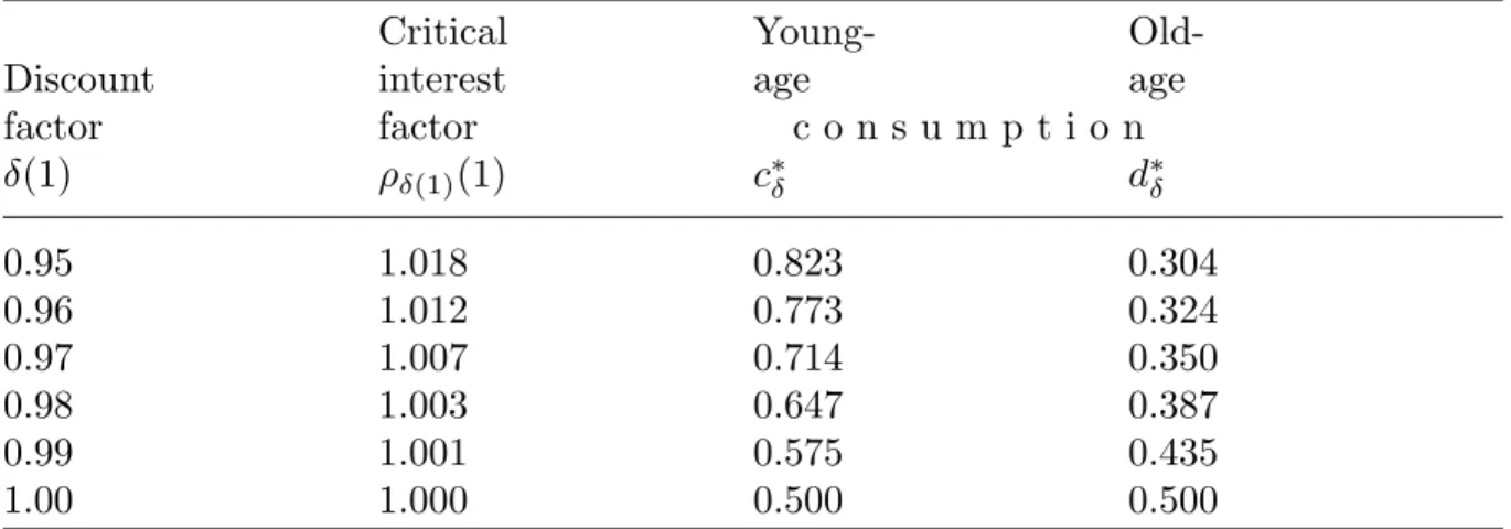
Notwithstanding all deficiencies of the model, it is worth demonstrating numerically how the critical value depends on the discount factor. Considering 30-year-long life- stages, our illustration applies only annual factors, derived from

δ(1) =δ^1/30 and ρ(1) =ρ^1/30.

For example, in the first line of Table 2, the annual discount rate of 5 percent defines a critical interest rate of 1.8 percent, and the ratio of old- to young-age consumption is equal to 0.37. But raising the discount rate, the critical interest rate quickly converges to zero and the consumption ratio slowly approximates 1.

Table 2. Autonomy and paternalism, annual factors

Critical Young- Old-

Discount interest age age

factor factor c o n s u m p t i o n

δ(1) ρ_δ(1)(1) c^∗_δ d^∗_δ

0.95 1.018 0.823 0.304

0.96 1.012 0.773 0.324

0.97 1.007 0.714 0.350

0.98 1.003 0.647 0.387

0.99 1.001 0.575 0.435

1.00 1.000 0.500 0.500

Remark. In the socially optimal mandatory pension system, c1 = 0.5 and d1 = 0.5.

2.3. Total intra- and intergenerational redistribution

At the end of this Section, unifying and simplifying the previous two models, we outline the model of Marxian communism: for inflexible labor supply and zero interest rate, full income redistribution is socially optimal. We do not need formulas: all incomes are taxed away and everybody receives the same transfer; the workers as tax returns and the pensioners as basic benefit.

These models are extremely simple, because they neglect at least one of the following complications: the intertemporality/heterogeneity of the population, the flexibility of labor supply and the possibility of underreporting earnings. Before entering the dis- cussion of these problems, we outline a general framework, assuming individuals with differing wage rates, discount factors etc.

3. General model

We distinguish the micro and the macro sides. The primitive quantities appearing in the model are generally positive (possibly zeros) and the functions are smooth. We assume that the population as well as the economy is stationary, moreover, there is no inflation.

3.1. Micromodel

Let vectorp of dimensionn+1 denote theindividual characteristicsof a person (e.g. his wage rate, discount factor etc.). Let vector q of dimensionN denote the characteristics of the government transfer system (e.g. contribution rate, accrual rate etc.). The employee works for a unit period and then is retired for another period, with length µ, 0 < µ ≤ 1. His young-age consumption is c, his per-period old-age consumption is d.

(Unlike in Subsection 2.2, at this stage we depart from the widespread but superfluous practice of identifying the lengths of the two periods in static models.) These variables depend on hisdecision vectorx of dimensionk. In the special models, the decisions are savings (including tax favored ones), labor supply and reported earnings.

Since one of the main reasons of having a mandatory retirement system is the indi- viduals’ shortsightedness, we single out the discount factor δ of the general characters, having thus p = (p, δ), where p is an n-vector. Then it is worthwhile distinguishing the per-period young- and old-age utility functions u1(p, q, x, c) and u2(p, q, x, d). The lifetime utility function is

U(p, δ, q, x, c, d) =u1(p, q, x, c) +µδu2(p, q, x, d).

In our abstract model, we have the following connection between the decisionxand the feasible consumption pair:

c=c(p, δ, q, x) and d=d(p, δ, q, x).

For example, since the government operates with a contribution rate τ, out of the full wage w only the net wage (1−τ)w flows into the young-age consumption. This can be further diminished by taking into account the restrained labor supplyl(<1) to (1−τ)wl.

The old-age consumption, in turn, primarily depends on the pension benefits: γ+βwl.

In addition, if the government subsidizes a voluntary pension scheme through a matching rate ϕ and finances the scheme by an earmarked tax with rate θ, then the subsidized saving r, the unsubsidized saving s and the earmarked tax θwl also reduce young-age consumption byr+s+θwland increase the old-age consumption byµ⁻¹ρ[s+ (1 +ϕ)r], whereρ is the interest factor. In the more sophisticated models, for given consumption, the young-age per-period utility is lower than its old-age counterpart, the difference being the labor disutility h(1−l).

Here we introduce the compositen+ 1 +N-dimensional vector of individual and the government characteristics P = (p, δ, q). Substituting the two consumption functions into the lifetime utility function yields the reduced utility function:

U^∗(P, x) =U(P, x, c(P, x), d(P, x)).

Following the neoclassical theory, we assume that every individual takes the govern- ment transfer system as given and maximizes his reduced utility function with respect to x:

U^∗(P, x)→max. Then we have

Theorem 3. a) For the locally optimal decision functionx(P), condition U^∗0_x(P, x) = 0

holds.

b) Assume that the k-order square matrix U^∗00_xx is strictly negative definite, then the matrix of rates of marginal change of x(P) is

x⁰(P) = [U^∗00_xx]⁻¹U^∗00_xP.

We shall need the balance function of the individuals, denoted by T(P, x). This determines the balance of the contributions and the benefits of type (p, δ) at the transfer system q.

The neutral system, where the balance is identically zero: T(P, x)≡ 0, is theoreti- cally interesting. Then the socially suboptimal decision xN(P) satisfies L⁰_x = 0, where the individual Lagrange-function is

L(P, x) =U^∗(P, x)−λ(P)T(P, x) and λ(P) is the appropriate Lagrange multiplier.

3.2. Macromodel

Until now we have only considered a single type with given individual characteristicsp and δ and government characteristics q. Now we introduce the heterogeneity of types.

Let E be the operator of expectation of the individual types (typically of wages and discount factors). Then the balance of the transfer system can be formulated as

ET(P, x(P)) = 0.

Note that this is already a general equilibrium model, where individual decisions depend on the transfer system and the balance of the latter also depends on the former.

In certain models, there is only a single transfer system (namely, the public pension) but in others, the tax system also appears. It is a question of choice to have either a unified or separated balances.

In our framework, the government maximizes apaternalisticsocial welfare function, where the individual discount factors are replaced by 1 and the transfer system is bal- anced. Also, the individual utility functions can be transformed by an increasing and concave function ψ, making the social welfare functionprogressive:

V(q) =Eψ[U^∗(p,1, q, x(p, δ, q))].

If ψ(U)≡U, then we receive pure utilitarianism.

Then the government chooses a vector of transfer characteristicsq^∗ such thatV(q) is maximal with respect to the balance equation(s). Again considering a local maximum, and relying on the method of Lagrange multiplier, we have

Theorem 4. A necessary first-order condition for a social optimum is L⁰_q =E

·

ψ⁰(U^∗)dU^∗

dq (p,1, q, x(p, δ, q))

¸

−νEdT

dq(p, δ, q, x(p, δ, q)) = 0 and ET(p, δ, q, x(p, δ, q)) = 0.

Remarks. 1. It is clear that for an N-vector q we have N independent scalar equations and ν is also an N-vector.

2. Note the contradiction between individual myopia and paternalism: V has para- meter values 1 and δ at the same time.

Comparing the social welfare provided by two transfer systems A andB, we cannot rely on the numerical values of the social optima, since the utility functions’ scales are also arbitrary. As in Subsection 2.1 above, we shall use an indirect method for comparison. Let e be a positive scalar and VX(e) be the social welfare assured by system X when all wages (rates) are uniformly multiplied by e. Then the efficiency of system A is e times that of B if VB(e) =VA(1).

What problems can be investigated with the help of such a family of models? A skeptic might say that such stylized models are useless. Luckily there are such or even more stylized models—or families of models—which give rise to strong conclusions.

At least such models are able refute certain qualitatively wrong ideas. For example, neutral systems are typically socially inferior to redistributive ones. On the other hand, excessive redistribution may undermine the efficiency of transfers so much that even the preferred types suffer from redistribution. In Sections 4 and 5 only specific models will be analyzed.

4. Specific models

In this Section we outline the specific models, transformed into an approximately com- mon form. Because of the lack of illuminating analytical results, we must often rely on numerical illustrations, and generally we rest satisfied with two types: denoted by L(ow) and H(igh). We have wageswL < wH, the types’ shares arefLandfH withfL+fH = 1.

The average wage rate is 1, implying wH = (1−fLwL)/fH. (Note, however, the con- tinuous wage distribution in Subsection 5.2 below). In the two-overlapping-generation models, numerically we work withµ= 1/2, i.e. the retirement period’s length is half of the working period.

Just as a warming-up, we return to the socially optimal contribution rate (of Sub- section 2.2), when saving is zero and µ ceases to be 1. Now

V1[τ] = log(1−τ) +µlog(µ⁻¹τ).

Therefore the socially optimal contribution rate is determined by V₁⁰[τ] =− 1

1−τ + µ

τ = 0, i.e. τ¯= 1 1 +µ⁻¹.

Ifτ >τ¯, thend > c, excess to be excluded. We shall call ¯τ maximal, corresponding to the perfectly far-sighted worker’s optimal saving rate. The corresponding net replacement rate is unitary: c=d.

4.1. Voluntary pension system

We start with the simplest special model, namely the interaction of mandatory and voluntary pension systems. The basic idea is simple: in economics, it is a commonplace that voluntary participation is generally better than mandatory one. But we have al- ready shown in Subsection 2.2 that in the case of life-cycle saving of myopic workers, some coercion may be needed. One hopes that this can be minimized, for example, by introducing voluntary pensions. Nevertheless, if one takes into account the tax expen- diture on tax-favored voluntary pension systems, then the attractiveness of this form is greatly diminished. Perhaps the existence of a cap on voluntary pension contributions already signals this effect.

As outlined in the introduction to the general framework, there is a worker earning wage w who pays a mandatory pension contributionτ w and will receive a proportional benefit b = µ⁻¹τ w when retired. In addition to this mandatory transfer, there is a possibility to contribute r to a voluntary system, matched by a factor ϕ by the government up to the cap ¯r. If the worker wants to save even more, he can save s without getting any matching. The factor of return to these private savings is ρ, i.e.

the old-age consumption becomes

d=µ⁻¹[τ w+ρ{(1 +ϕ)r+s}].

Note, however, that this matching must be covered by proportional earmarked taxes, θw. Therefore the worker’s consumption reduces to

c=w−(τ +θ)w−r−s.

In this Section we neglect the real interest rate: ρ= 1 and work with CRRA rather than Cobb–Douglas-utility function: u(c) =σ⁻¹c^σ, where σ <0. (For σ = 0, we would obtain the log-utility function! Note that in Subsection 2.2, the optimal saving s_δ was independent of the interest factor ρ, showing degeneracy!) Then for positive savings, the optimal consumption pair satisfy

d =cD(δ, ϕ), where D(δ, ϕ) = [δ(1 +ϕ)]^1/(1−σ). For zero saving, d > cD(δ, ϕ).

We assume that the lower paid have a lower discount factor than the higher paid have:

0≤δ_L< δ_H ≤1.

We have two balance equations.

Pension balance:

µβEw =τEw, i.e. τ =µβ.

Earmarked tax balance:

ϕEr =θEw.

It is evident that no rational worker would save normally before exhausting the possibilities of voluntary contributions in [0,r].¯

We compare three idealized systems: (i) thepurely mandatorysystem, (ii) theasym- metric system, where only the far-sighted participate and (iii) the symmetric system, where both types participate proportionally to their wages. We shall see that the sym- metric system is socially superior to both the pure mandatory system and the asym- metric one, which in turn are roughly equivalent.

To save space, here we only discuss the asymmetric voluntary system, and confine attention to a single case from Theorem 3 of Simonovits (2009). As a preparation, let us denoteδ^o the government implicit discount factor, implying the mandatory contribution rate τ, as an individual optimum (τ = sδ^o). Then let ϕL be that positive scalar, for which δL(1 + ϕL) = δ^o, i.e. that matching rate at which type L is just without a voluntary contribution.

Theorem 5. If the matching rate is low enough, 0 < ϕ ≤ ϕL and the cap on voluntary contribution is high enough:

¯

r > r_H(ϕ) = [D(δ_H, ϕ)(1−τ)−µ⁻¹τ]w_H D(δH, ϕ)(1 +fHϕwH) + (1 +ϕ)µ⁻¹, then type H’s optimal contribution is equal to rH(ϕ), while sH = 0.

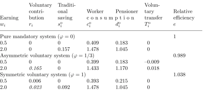
To illustrate our findings numerically, we choose σ = −1, δ_L = 0.15; δ_H = 0.5 (annually δL(1) = 0.939; δH(1) = 0.977). The government contribution rate τ = 0.183 corresponds to a medium discount factor δ^o = 0.2 (annually δ^o(1) = 0.948). To have simple algebra, the cap in each voluntary system is to be equal to H’s voluntary contribution (italicized in Table 3). To amplify the effects, we choose a rather unequal wage distribution: fL = 2/3 andfH = 1/3 withwL = 0.5 andwH = 2. Table 3 presents a numerical illustration.

Table 3. Comparison of combinations of mandatory and voluntary pensions

Voluntary Traditi- Volun-

contri- onal Worker Pensioner tary Relative

Earning bution saving c o n s u m p t i o n transfer efficiency

wi ri s^o_i c^o_i d^o_i T_i^o e

Pure mandatory system (ϕ= 0) 1

0.5 0 0 0.409 0.183 0

2.0 0 0.157 1.478 1.045 0

Asymmetric voluntary system (ϕ= 1/3) 0.989

0.5 0 0 0.399 0.183 –0.009

2.0 0.165 0 1.433 1.170 0.018

Symmetric voluntary system (ϕ= 1) 1.038

0.5 0.006 0 0.393 0.215 0

2.0 0.023 0.092 1.478 1.045 0

(i) The pure mandatory system is only displayed as a benchmark, with relative efficiency 1. Note the unacceptably low old-age consumption of the myope: d^o_L = 0.183.

(ii) The mandatory pillar supplemented with an asymmetric voluntary pillar only makes things a little bit worse because the matching rate is too low to help the myope (ϕ = 1/3) and the ceiling on voluntary contribution is high enough (¯r = 0.165) to allow the far-sighted to appropriate all the benefits. The earmarked tax rate creates a net transfer from the myopes to the far-sighted. The young-age consumption of the former slightly diminishes, just to help raise the far-sighted’s old-age consumptions. The pure mandatory pillar can achieve the same social welfare as the asymmetric voluntary system with 1.1 percent lower wages.

(iii) The mandatory pillar supplemented with a symmetric voluntary pillar redresses the injustice: the matching rate is raised to 1, while the ceiling is drastically lowered to 0.023. The myope’s old-age consumption rises now fromd^o_L= 0.183 to 0.215, the young- age consumption drops from c^o_L = 0.409 to 0.393, while c^o_H and d^o_H remain invariant.

The pure mandatory pillar can only achieve the welfare of the symmetric voluntary system by increasing wages uniformly by 3.8 percent. Note, however, that this is the same as a 1.2 + 1.2 = 2.4 percent point increase of the mandatory contribution rate!

4.2. Cap on the contribution base

In most countries, workers do not pay pension contributions after the earning above the so-called contribution base cap, shortlycap. In the Introduction, we promised to model a neglected function of the cap: it effectively limits the ratio of the contribution to the earnings, reducing the presumed adverse efficiency impact of mandatory saving: this is the basis of the present model. We shall see that in our specification, the cap has hardly any welfare impact in the relevant interval but is socially superior to the capless case.

Our starting point is the cap ¯wand the covered total wage ˆw= min(w,w). Then the¯ contribution is equal to τw. We introduce the covered net wage and the correspondingˆ benefit:

ˆ

v= (1−τ) ˆw and b=βv.ˆ

We shall also need the effective contribution rate, defined as the ratio of contribution to wage:

˜ τ = τw¯

w if w >w¯ and τ˜=τ if w ≤w.¯

Obviously, for a wage higher than the cap, the effective contribution rate is lower than the statutory one: w >w¯ implies ˜τ < τ.

We only display the most important formulas. We should distinguish again two cases: the saving intention is either (i) nonnegative or (ii) negative.

To determine the optimal saving, we need the Cobb–Douglas-lifetime utility function U(w, δ, c, d) = logc+µδlogd.

Inserting the consumption functions

c=w−τwˆ−s and d=βvˆ+ρµ⁻¹s, we obtain the derived utility function

U^∗(w, δ, s) = log(w−τwˆ−s) +µδlog(βvˆ+ρµ⁻¹s).

Introducing the cap-dependent net earning w−τw¯ and taking the derivative by s and equating it to zero; yields

1

v−s = δρ b+µ⁻¹ρs. Hence we have the following result.

Theorem 6. In a pension system with the cap-dependent net earningw−τw, the¯ optimal saving intention is

sⁱ = δρv−b (δ+µ⁻¹)ρ.

Ifδρv≥b, thensⁱ ≥0, i.e. s^o =sⁱ and d^o =δc^o. Otherwise, if δρv < b, thensⁱ <0, i.e. s^o = 0 and d^o > δc^o.

In our paternalistic framework, the government maximizes the expected value of U^∗[w,1] = log(w−τw¯−s^o) +µlog(βvˆ+ρµ⁻¹s^o)

rather than EU^∗[w, δ]. That is,

V(τ,w) =¯ EU^∗[w,1].

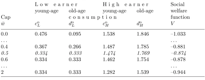
We confine our numerical illustrations to the 2-type case. Input data: The com- pounded discount factors for 30 years are δ_L = 0.1; and δ_H = 0.6 (annually δ_L(1) = δ_L^1/30 = 0.926..andδ_H(1) =δ_H^1/30 = 0.983..); while the interest factor isρ = 2 (annually ρ(1) = 2^1/30 = 1.0234..). By theoretical and numerical reasoning, the socially optimal contribution rate τ^o = 0.333. Table 4 shows that the social welfare function increases with the cap until wL and then it drops. The key to the solution is to be found in the consumption of the lower paid: d^o_L( ¯w), which grows until ¯w reaches w_L (italicized row), beyond which it only reduces the possibilities of the high-earners.

Table 4. The impact of cap on the social welfare

L o w e a r n e r H i g h e a r n e r Social young-age old-age young-age old-age welfare

Cap c o n s u m p t i o n function

¯

w c^o_L d^o_L c^o_H d^o_H V

0.0 0.476 0.095 1.538 1.846 –1.033

. . . . . .

0.4 0.367 0.266 1.487 1.785 –0.881

0.5 0.334 0.333 1.474 1.769 –0.874

0.6 0.334 0.333 1.462 1.754 –0.878

. . . . . .

2 0.334 0.333 1.282 1.539 –0.944

Remark. τ^∗ = 0.333, ¯w^∗ = 0.5.

The wages should be uniformly increased by 11.1 and 4.6 percent in the no-pension or the no-cap pension system respectively to have as high social welfare as with the socially optimally capped pension system.

4.3. Redistribution with flexible labor supply

This istheclassical model, where the two introductory models (Subsections 2.1–2.2) are modified, unified and the third (Subsection 2.3) is generalized.⁹ Here the labor supply is flexible and is influenced by the personal income tax rate and the forced saving for old- age. To keep the model as simple as possible, there is no private saving and the personal income taxθwl is copied from Subsection 2.1 but the basic incomeγ is extended to the old. We recall some earlier notations and formulas: τ = contribution rate,θ = personal income tax rate, t = τ +θ = transfer rate and ¯t = 1−t = the net-of-transfer rate.

Furthermore, l = labor supply. The pension benefit in turn consists of two parts: flat benefit γ and the proportional benefit βwl, where β is the so-called accrual rate (or equivalently, marginal replacement rate) and wl is the total earning. Hence the total benefit is b(wl) =γ+βwl. We display the consumption pair:

c=γ+ ¯twl and d=γ +βwl.

Without proof, we give the necessary condition for individual optimality.

Theorem 7. The necessary condition for the optimal labor supply is

¯tw

γ+ ¯twl − ξ

T −l + δµβw γ +βwl = 0.

With rearrangement, a quadratic equation is obtained:

a2l²+a1l+a0 = 0, where

a2 =−(1 +ξ+δµ)¯tβw²,

a1 = ¯tw(T βw−γ)−ξw(γβ+ ¯tγ) +δµβw(¯twT −γ), and

a0 = ¯twT γ−ξγ²+δµβwγT.

We shall consider two special cases: (i) the proportional pension system (P) without redistribution: γ = 0 and (ii) the pure flat benefit system (F): β = 0. Here the optimal labor supplies are as follows:

l^P₀ = T

1 +ξ < l^P = (1 +δµ)T

1 +ξ+δµ < T and 0< l_w^F = T −ξγ/(¯tw) 1 +ξ < l^P₀,

wherel₀^P is the labor supply of Feldstein’s myopes (δ= 0). The unified balance condition is as follows:

tE(wl) = (1 +µ)γ +µβE(wl), i.e. γ = (1 +µ)⁻¹(t−µβ)E(wl), t ≥µβ.

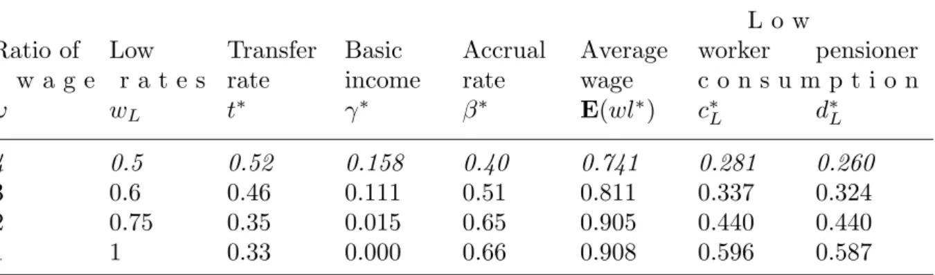
We only illustrate the impact of wage rate inequality, i.e. reduce the ratio ω = wH/wL from 4 to 1. It is to be expected that the socially optimal transfer rate is

9 Among the models surveyed, this is the closest to Cremer et al. (2008)!

dropping along, but only numerical calculations, displayed in Table 5, give the measures:

namely the socially optimal transfer rate drops from 0.52 to 0.33 and through the rise of labor supply, the average wage rises from 0.74 to 0.91. But it is quite surprising that the optimal redistribution among workers disappears well before reaching wage rate equality, namely slightly below ω = 2 (exactly at 1.8)! At the same time, the accrual rate β^∗ steeply rises and reaches the value of the optimal proportional system. We cite Table 4 from Simonovits (2012d).

Table 5. The impact of earning inequality on the social optimum L o w

Ratio of Low Transfer Basic Accrual Average worker pensioner w a g e r a t e s rate income rate wage c o n s u m p t i o n

ω wL t^∗ γ^∗ β^∗ E(wl^∗) c^∗_L d^∗_L

4 0.5 0.52 0.158 0.40 0.741 0.281 0.260

3 0.6 0.46 0.111 0.51 0.811 0.337 0.324

2 0.75 0.35 0.015 0.65 0.905 0.440 0.440

1 1 0.33 0.000 0.66 0.908 0.596 0.587

Remark. µ= 0.5, δL = 0.4 andδH = 0.7.

4.4. Underreporting wages

One of the most important problems of public economics, especially during transition (from socialism to capitalism) is as follows: how to achieve income redistribution in such a way that the lower income people do not starve and the higher income people do not hide too much of their incomes? Using the tax morale, mentioned in the Introduction, endogenizes underreporting of labor incomes. Excluding the old-age, we had already been able to derive quite sharp analytical results in the generalization of Subsection 2.1 (cf. Simonovits, 2012b). But extending the analysis to the second stage, we have to be content with more modest results.

We keep the notations of Subsection 4.3, except for wl is replaced byreported wage v. We choose the simplest progressive tax system, where every worker pays a linear earning tax θv and receives a lump-sum return ε. Thus the net tax is equal to θv−ε.

The pension benefit in turn consists of two parts: flat benefit α and the proportional benefitβv, whereβ is the so-called accrual rate. Hence the total benefit isb(v) =α+βv.

In addition to forced savings via the pension system, workers also can save privately, its value is denoted by s, there is no interest: ρ= 1. We display the consumption pair:

c=w−tv+ε−s and d=α+βv+µ⁻¹s.

In the spirit of the tax morale literature, we introduce the tax morale parameter m, influencing the subjective utility of the worker underreporting his true earning w:

z(w, m, v) =m(logv−v/w).

Due to the linear correction term, z(w, m,·) has a maximum at v=w. In fact, z⁰_v(w, m, v) = m

v − m w >0

if and only if 0< v < w, i.e. the overreporting individual is not rational.

The other terms of the lifetime utility function are standard and have been intro- duced in Section 3:

u1(c) = logc and u2(d) =δlogd.

In sum, the total individual utility function is

U(w, m, δ, c, d, v) = logc+m(logv−v/w) +µδlogd.

Executing the substitutions and equating the partial derivatives (with respect to wage reporting and saving) to zero, yield the individual optimum. Because savings cannot be negative, we must distinguish again between two cases: a) the saving intention is nonnegative or b) negative. In the former case, the saving intention is realized (slack credit constraint); in the latter case, the actual saving becomes zero (binding credit constraint). We only consider here the former case.

Theorem 8. Under our assumptions, if the worker has a slack credit constraint, then the individually optimal young-age consumption c is the positive root of the fol- lowing quadratic equation:

h2c²+h1c+h0 = 0, where t1 =t−µβ and

h2 =m(1 +µδ), h1 =t1(1 +µδ)w+t1mw−m(w+µα+ε), h0 =−t1w(w+µα+ε).

This individually optimal worker’s consumption defines the other components like reported wage v.

To get rid of the mathematical difficulties of the tax balance equation, we assume the existence of a positive net average tax ¯a = E(θv−ε). Furthermore, the individual utility is enhanced by the utility of public goods, modeled as

q(¯a) = (1 +µ)κlog ¯a,

where κ is the coefficient of relative utility of public goods to that of young-age con- sumption.

At this point, we must consider the pension balance equation:

τEv=µEb(v).

We arrived to a relatively simple general equilibrium model mentioned in Section 3.

We display two numerical calculations, where the tax morale is relatively weak and strong, respectively: a dark grey economy with m= 0.5 and a light grey economy with

m = 2. For the relative utility parameter κ = 1/3, we determine the socially optimal values of the transfer system.

Unlike in light grey economy, in the dark grey economy, the socially optimal basic income is always zero, therefore Table 6 has one column less than Table 7. Citing Table 4 in Simonovits (2009b) we see that the higher the flat component, the lower the average reported wage and consequently, the lower the social welfare, assuming that the government chooses socially optimal tax rates. Repeating our warning again: there is not much sense in differences between the values of social welfare functions, rather we must measure the decline by consumption equivalence. For example, let e > 1 be such a scalar that by multiplying both types’ wages with it, the social welfare of a flat component α = 0.2 becomes identical to that of the original proportional system. We obtain e = 1.03, i.e. the economy should have wages uniformly higher by 3 percent to achieve the original welfare of the proportional system in the foregoing flat system.

Table 6. An optimal system with a given flat benefit, dark grey economy, m= 0.5

Contri- Marginal Average

Flat bution Tax replace- Reported net Social

benefit rate rate ment rate wage tax welfare

α τ^o θ^o β^o ¯v^(P) ¯a V

0.00 0.22 0.28 0.440 0.547 0.102 –3.108

0.04 0.35 0.29 0.620 0.500 0.097 –3.113

0.08 0.37 0.29 0.568 0.466 0.090 –3.124

0.12 0.36 0.29 0.447 0.439 0.085 –3.140

0.16 0.36 0.29 0.331 0.411 0.079 –3.161

0.20 0.35 0.29 0.181 0.385 0.074 –3.185

Turning to the light grey economy (Table 5 in Simonovits 2009b), the purely propor- tional system is less efficient than the optimally redistributive one. In our specification, the average reported wage is also a decreasing function of flat component, but its im- pact is weak enough that the proportional benefit disappear around α = 0.28, before the system reached the optimum atα = 0.32. In the purely proportional system, wages should be increased uniformly by 2.1 percent to achieve the same social welfare as in the social optimum with basic benefit α= 0.32.

Table 7. An optimal system with a given flat benefit, light grey economy, m= 2

Contri- Net Marginal Average

Flat bution tax Basic replace- Reported net Social

benefit rate rate income ment rate wage tax welfare

α τ^o θ^o ε β^o v¯^(F) a¯^(F) V^(F)

0.00 0.26 0.40 0.10 0.520 0.732 0.128 –4.810

· · · · · ·

0.20 0.26 0.36 0.07 0.239 0.712 0.124 –4.773

0.24 0.21 0.27 0 0.094 0.735 0.132 –4.772

0.28 0.20 0.27 0 0.013 0.724 0.130 –4.767

0.32 0.22 0.28 0 0 0.707 0.132 –4.755

0.36 0.25 0.26 0 0 0.703 0.122 –4.760

0.40 0.28 0.24 0 0 0.699 0.112 –4.773

5. Original specifications

As was mentioned in the Introduction, in displaying the specific models in Section 4, to approach a common framework, we have frequently deviated from the original specifi- cations. Here we present some original ones, which shed some light on the sensitivity of the models as well.

5.1. Discounted Leontief utility and cap

As is known, the additive discounted utility function, introduced by Samuelson (1937) and specified as CRRA, contains the discounted Cobb–Douglas and the undiscounted Leontief utility functions as special cases. But following the spirit of Shane, Loewenstein and O’Donoghue (2002), we gave up the additivity assumption, and to help analytical discussion of the contribution cap, originally we chose a specific utility function, called discounted Leontief utility function:

U(w, δ, c, d) = min(δc, d).

Note that this lifetime utility function is not age-additive, and surprisingly it is the young- rather than the old-age consumption which is discounted. Note, however, that for any positive saving, at the optimum, δc =d, i.e. the lower the discount factor, the lower the old-age consumption. An additional advantage of this specification lies in that for reasonable choice of the contribution rate, c > d, i.e. U(w, δ, c, d) = d, yielding a simple social welfare function: V =Ed. Simonovits (2013) conjectured that the unitary replacement rate is socially optimal.

We only display the most important formulas. Again, we should distinguish two cases: the saving intention is (i) nonnegative or (ii) negative.

Ad (i). At the optimum, δc^∗ = d^∗, i.e. δv −δs = b+µ⁻¹ρs yielding the saving intention sⁱ = (δv−b)/(δ+µ⁻¹ρ), which is realized of and only if δ ≥δ_τ =µ⁻¹τw/v.ˆ Then c^∗₁ = (ρv+µb)/(µδ+ρ).

Ad (ii). If sⁱ <0, then s^∗₂ = 0, i.e. c^∗₂ =v and d^∗₂ =b.

Here we confine our numerical illustrations to the 3-type case. Input data: fL = 0.7;

fE = 0.25 andfH = 0.05, wages: wL= 0.7; wE = 1.3 andwH = 1.7. The compounded interest factors for 30 years are δL= 0.215; δE = 0.545 andδH = 0.97; at annual level:

δL(1) = 0.977; δE(1) = 0.988 and δH(1) = 0.999. The socially optimal contribution rate τ^∗ = 0.333 and the corresponding cap ¯w^∗ = wE. Table 2 of Simonovits (2012a) is reproduced here.

Table 8. The impact of cap on the social welfare, 3 types, Leontief

Medium High Social

Cap c o n s u m p t i o n welfare

¯

w d^o_E d^o_H V =Ed

1.0 0.666 1.198 0.626

1.1 0.733 1.185 0.641

1.2 0.799 1.172 0.655

1.3 0.866 1.159 0.670

1.4 0.866 1.146 0.668

1.5 0.866 1.133 0.666

1.6 0.866 1.120 0.664

1.7 0.866 1.132 0.666

Remark. τ^∗ = 0.333, ¯w^∗ = 1.3.

Note that raising the cap from 1 to the medium wage 1.3, the weighted increase in d^o_E is greater than the weighted decrease in d^o_H. Above w_E, the further rise in ¯w only diminishes d^o_H, without raisingd^o_E.

5.2. Pareto-distribution

Though in our survey, the earning distribution is generally discrete, with two or three types, now we present a more realistic, continuous earning distribution named after Wilfredo Pareto (cf. Diamond and Saez, 2011). The distribution function is given as

F(w) = Z _w

wm

f(ω)dω = 1−w^σ_mw^−σ, where w ≥wm,

σ > 1 and wm > 0 is the minimal earning. Normalizing the average wage to 1, the minimum wage is wm = (σ−1)/σ.

Selected numerical values are displayed in Table 9. Note that the lower 50 percent of earners have only 25 percent of the total earnings, while the upper 3 percent of earners have 17 percent.