We do this in the physical coordinate system r and on the basis of complete physical quantities. These are the density ρ(r, t) at a location r, the corresponding total velocity u(r, t) and the total gravitational potential Φ(r, t) as well as the pressure P(r, t) of the medium. .
Perturbations: from physical to comoving coordinates
Due to the expansion of the background, the velocity perturbations of the FRW universe are gradually attenuated: the additional displacement associated with the peculiar velocity will bring the motion of a particle more and more in line with the background Hubble expansion, and the motion of the particle becomes more and more in line with the expected Hubble expansion. The only way to maintain and increase velocity perturbations is therefore the right-hand source term, the influence of the gravitational field.
Linear Evolution
One can always find large scales where the density and velocity perturbations still exist in the linear regime. In the following sections, we will deal with a few of the most relevant situations with linear perturbation development.
Matter-Dominated FRW Universes: Linear Perturbations
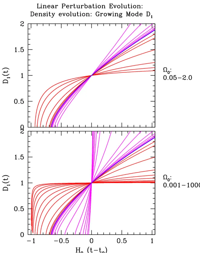
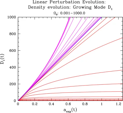
From the three fluid equations we can directly deduce the time evolution of the density perturbation δ(x, t). The density values of the corresponding density contours evolve, all developing at the same rate, the growth factor D(t).
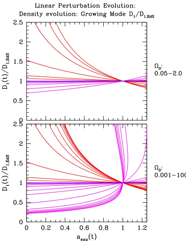
Linear Density Growth factors in Matter-dominated FRW Universes
Einstein-de Sitter Universe
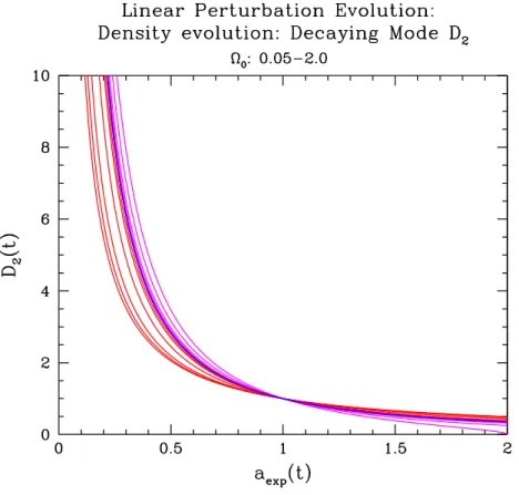
Note that in this particular case of an Einstein-de Sitter universe, the growth is proportional to the expansion factor of the universe. The second solution, on the other hand, leads to a continuously decreasing density: the original density contrast decreases with time. Once its share (between growth and decay modes) in the initial density fluctuations has been established, it is often disregarded in further considerations in the evolution of the structure: its share gradually fades away and will no longer be noticeable in the current era.
By choosing this convention, the spatial functions ∆1(x, t) and ∆2(x, t) come to correspond to linearly extrapolated density fluctuations. They are the density values that a fluctuation would have if it had continued to grow linearly up to the current epoch (which it usually does not). As for the contribution from the decay state, it would have to be very small indeed today to prevent it from being greater than unity in the early universe.
In summary, we find that the general solution for the linear evolution of a density fluctuation in an Einstein-de Sitter universe is given by the sum of a growing solution, specified by the normalized density growth factor D1(t) =a(t) , and a decaying solution specified by D2(t)∝t−1.
Empty Universe
In this case too, we can identify two solutionsδ1 andδ2, and each of them can be separated into a spatial and a temporal part. Interestingly, the solution δ1(x, t) stops instead of growing: density growth freezes out and the structure retains the current configuration. On the other hand, the solution with decay state behaves the same as in an Einstein universe.
When we extrapolate back in time, we see that the consequence of such a scenario in terms of the formation of today's structure is that it must have been in place in the primordial Universe. Apparently, this would be difficult to reconcile with our knowledge of the early Universe (in particular, the isotropy of the cosmic microwave background). However, after noting that an empty Universe can be considered the asymptotic state of an evolving open FRW Universe, we can conclude that the present structure has been in place since a much earlier cosmic epoch.
This era is the time when a not yet empty universe evolved into a freely expanding empty universe.
General Matter-Dominated FRW Universes
This results in a lower value of the Hubble dragterm ˙a/a. 42) we can easily estimate that this results in an acceleration of the density evolution. Perhaps unsurprisingly, structure grows faster in a closed universe, mainly due to the higher background density of the universe and the corresponding higher mass content of density fluctuations. In an open universe we see the opposite, the growth of structure will take place less quickly than in an Einstein-de Sitter universe.
For a(t) ≫ 1 the x(t) term becomes dominant over all, so the open Universe has proceeded to free expansion,. The growth of the linear density in an open universe proceeds from a primordial situation in which it resembles that in an Einstein-de Sitter Universe, D(t)∝a(t), to a halt in the growth of structure similar to in a free expansion. Empty universe, D(t) = const. If we lived in an open Universe at the time of the transition, this would mean Ω0 ≈0.5.
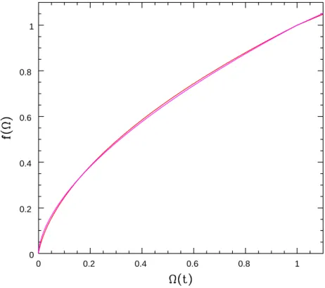
An alternative expression for the growth mode solution D1(t) is in terms of the development angle Φu.
Linear Perturbations: FRW Universe with Dark Energy
FRW Universes containing Matter and Cosmological Constant
In the presence of a cosmological constant in a generally curved FRW universe, the linear growth of density perturbations in the matter distribution can be evaluated directly via an integral expression. However, in the presence of a significant radiative contribution to the cosmic energy density, matter evolution and radiative perturbations are coupled (see Section 9 ), complicating the analysis somewhat. In Section 9 we will focus on the linear evolution of radiative perturbations (larger than the Jeans mass).
Here we will focus on the evolution of matter perturbations in a general FRW Universe, filled with matter and a cosmological constant, with a general curvature (see also Hamilton 2000 ). Multiplying the evolution equation of H by D(t) and subtracting H(t) times the equation for D(t) we have. The linear perturbation growth factor D(t) can be calculated for any FRW Universe with matter and a cosmological constant - specified by the parameters Ωm,0 and ΩΛ,0 - by inserting the expression for the evolution of the Hubble parameter 79 into the integral above the expression and calculating the integral.
For the relative growth factorg(t)≡D(t)/a(t) – relative to the equivalent Einstein-de Sitter universe – we find (see for example Lahav & Suto 2003).
Linear Radiation Perturbations
CMBFAST, the code for calculating temperature perturbations in the cosmic microwave background, does just that. In the first subsection 9.1, we will study the evolution of radiation disturbances in this regime in which radiation is the only cosmic component of interest. Near the epoch of radiation-matter equivalence and until the epoch of recombination and consequent decoupling between matter and radiation, radiation remains a significant factor in the evolution of perturbations.
In the continuity equation and the Euler equation, we must take into account a pressure inertia. This is a far more restrictive assumption than in the case of the matter-dominated universe. The analysis presented in this section is therefore hardly realistic, there are almost no radiation disturbances whose development is not affected by the pressure in the radiation fluid.
The perturbation evolution equation for radiation is therefore almost equivalent to that for linear perturbations in the matter distribution.
Gravity Perturbations
Gravitational Potential Perturbations
Note that density perturbations δ(x) throughout the observable universe (i.e. within the horizon) contribute to the potential. In reality, the spatial distribution and nature (magnitudes) of the density perturbations will determine the extent of the cosmic volume that has a significant dynamical influence. The integral expression also allows to immediately identify the time evolution of the potential disturbance.
As photons climb out of the potential hole, they are redshifted, causing the CMB temperature to cool. Since in an Einstein-de Sitter universe φ remains constant in time, the integral of the temperature shift along the photon path leads to the measured temperature shift relative to the global CMB temperature. Therefore, the map of measured CMB temperature fluctuations can be directly translated into a map of gravitational potential perturbations during the recombination period (and thus into a map of the corresponding density fluctuations).
For the same, by evaluating the density fluctuations along the path of a CMB photon, one can try to find out the evolution of the potential growth factor Dφ(t).
Peculiar Gravity
As a photon (microwave background) travels through space from the surface of last scattering, around the time of recombination, to a telescope/detector on planet Earth, some 12.7 Gyrs later, its frequency will change as it travels along its path. breaks through the potential. landscape. The temperature shift is the combined effect of the corresponding gravitational redshift and time dilation (see Chapter 1) and is known as the Sachs-Wolfe effect. In other words, by measuring the integrated temperature shift along the photon's path, the so-called integrated Sachs-Wolfe effect, one can find the corresponding potential evolution.
Instead, the inverse relation can potentially be used to infer basic cosmological parameters, hinting at the exciting possibility of directly measuring the value of the cosmological constant. Both the equation for gravitational potential perturbations (111) and that for the peculiar gravitational acceleration (120) should be considered as the core of the theory of gravitational instability. It might be worth noting that in almost all situations of linear structure formation, the corresponding anomalous gravitational accelerations appear to decrease with time.
However, it is mainly a consequence of the continuous expansion of the universe and the associated increase in cosmic distances.
Peculiar Velocity
An interesting observation is that in the linear regime we find that the Lagrangian time derivative of the peculiar velocity vis is equivalent to the Eulerian time derivative of v, due to the discarding of the second order term. The second of these equations shows that the curl portion of the velocity decays as v⊥ ∝ 1. This is a clear illustration of the observation that one can deduce the global properties of a system by studying its perturbations.
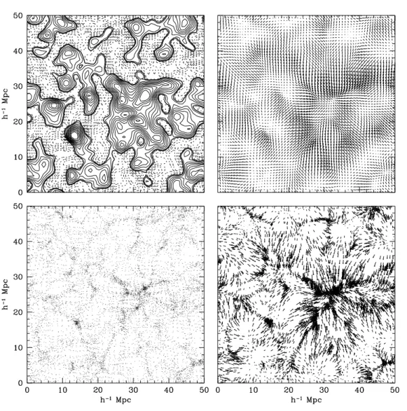
If it were indeed an unbiased reflection of the cosmic density field, this would mean that the galaxy distribution is a Poisson sample of the underlying continuous density δ(x) and that its local number density n(x) is a direct reflection of δ(x) ), This means that includes all structures whose influence is important for the dynamics of the local volume Vgalvel, in which we measured the velocities. Since we do not have any convincing theory of galaxy formation, we cannot be certain about the connection between the distribution of matter and the distribution of galaxies.
It is not inconceivable that something like this could be a feature of the galaxy formation process. One can attempt to determine Ωm by determining the peculiar velocities of galaxies and combining this with mapping the spatial matter distribution in the dynamically relevant region (i.e. once it has become possible to determine the peculiar velocities of galaxies relatively accurately, from from the mid-eighties of the last century onwards, astronomers had a way to determine the cosmic matter density.
Linear Theory: Fourier Mode Evolution
We must emphasize that the practical complications associated with measuring special speeds are 'in principle' enormous.