Model predictive control of a Kaibel distillation column

Unfortunately, at the time of the diploma work, the laboratory column was not available for MBK. A single-layer MPC and a supervised MPC approach were described, implemented and tested on the simulation model of the column.

A BBREVIATIONS

I NTRODUCTION

• Motivation
• THE KAIBEL DISTILLATION COLUMN 3
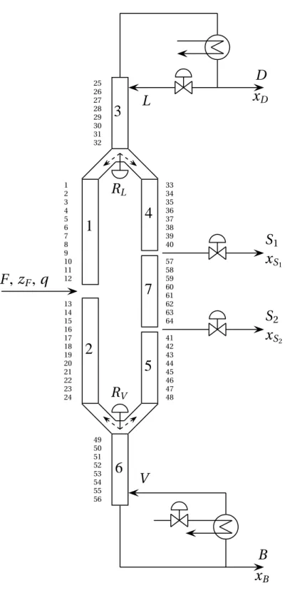
• The Kaibel distillation column
• Model predictive control
• Project scope
• THESIS OUTLINE 5
• Thesis outline
• Source code

One of the main challenges associated with using the Kaibel distillation column is in the field of control. As part of earlier work, a mathematical model was made for computer simulations of the Kaibel distillation column.

B ACKGROUND

• Research at BASF
• Work by PhD fellow Jens Strandberg
• FINAL YEAR PROJECT WORK FALL 2008 9
• Final year project work fall 2008

In the control part of the project work, decentralized control was presented along with model predictive control (MPC). Since decentralized control requires the process to have little interaction, an interaction analysis was conducted during the project work.

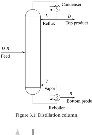
I NTRODUCTION TO DISTILLATION AND THE

K AIBEL DISTILLATION COLUMN

• Distillation theory
• DISTILLATION THEORY 13
• Equations used in distillation
• The Kaibel distillation column
• DISTILLATION MODELING 15
• Distillation modeling
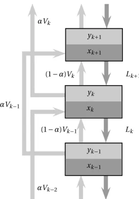
• DISTILLATION MODELING 17 A single simulation step in the simulation model
• LINEARIZED AND REDUCED MODEL 19
• Linearized and reduced model
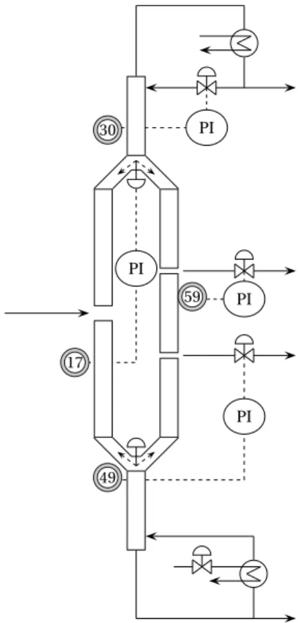
• Control of the distillation column
• CONTROL OF THE DISTILLATION COLUMN 21
• CONTROL OF THE DISTILLATION COLUMN 23
• CONTROL OF THE DISTILLATION COLUMN 25

The material balance is then dNi,k. 3.2) The number of moles of a component on a stage is equal to Mkxi,k, where Mk is the total number of moles on stagek. If the model simulates using the nominal values ​​for inputs as given in Table 3.2, the nominal values ​​will be for the four product compositions.

P ROBLEM STATEMENT

• Model extension
• Model predictive control
• EVALUATION OF ALTERNATIVE MPC APPROACHES 29
• Evaluation of alternative MPC approaches

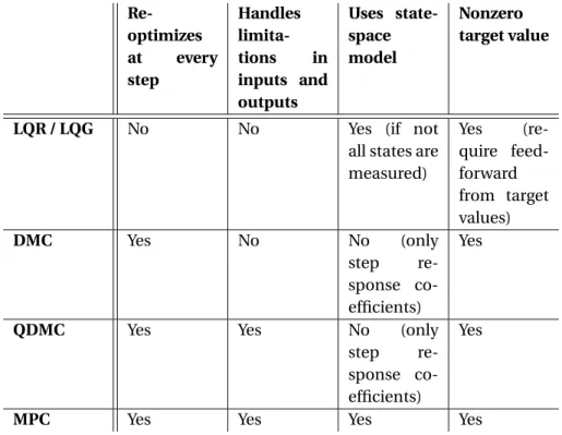
The author aims to implement, test and compare three different MPC designs for controlling the Kaibel column model. There are several MPC approaches; therefore, a brief discussion is necessary to evaluate these alternatives for controlling the Kaibel distillation column. 1When the unbounded objective function is convex, it is easy to find the global optimum because it is located at the point where the first derivative of the objective function is zero.

For a non-convex optimization problem, things get more difficult because the first derivative of the objective function is zero several places and the global optimum is much harder to find.

M ODEL EXTENSION

• Vapor bypassing
• Simulations with vapor bypassing
• SIMULATIONS WITH VAPOR BYPASSING 33
• SIMULATIONS WITH VAPOR BYPASSING 35

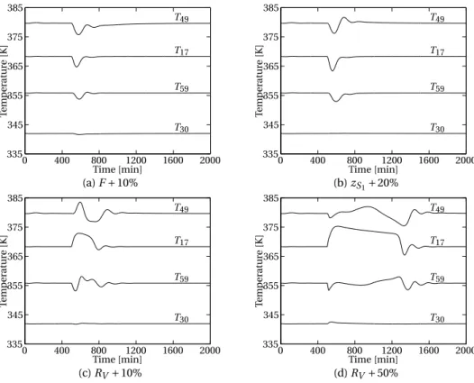
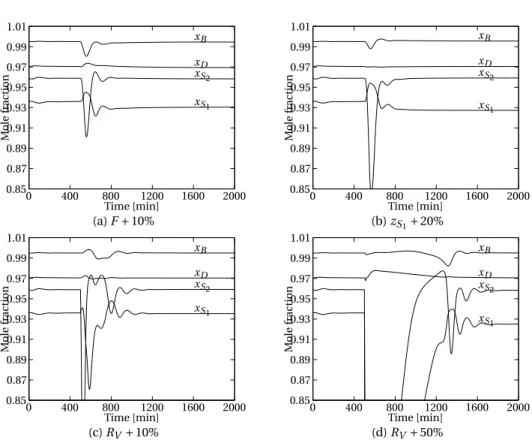
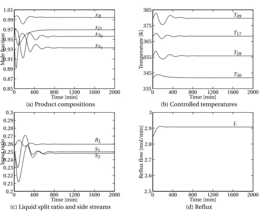
The inclusion of vapor bypass keeps the number of column stages the same, but introduces an efficiency parameter (α) that describes insufficient mixing of the vapor at the column stages. This is to see what the controller does to prevent the vapor from bypassing to reach the set temperatures. The liquid split ratio and the two side streams remain at approximately the same values, but the reflux increases (Figure 5.4d).

As the profile moves to the left, the column appears to become much hotter from a regular plot of temperature versus time.

I NTRODUCTION TO MODEL PREDICTIVE CONTROL

• Linear quadratic regulator
• DYNAMIC MATRIX CONTROL 39
• Dynamic matrix control
• MODEL PREDICTIVE CONTROL 41
• Model predictive control
• MODEL PREDICTIVE CONTROL 43
• MODEL PREDICTIVE CONTROL 45
• LQR, (Q)DMC and MPC comparison
• Variants of model predictive controllers
• IDENTIFICATION OF MODEL 47
• Identification of model
• IDENTIFICATION OF MODEL 49
• Control layers

The output in the future time k+l (l>0) can be written as the sum of the effects of future and past moves. After this horizon, the input can be set to be constant or proportional to the state (eg use LQR gain). These can be chosen arbitrarily, but it is required that Q≥0 and R>0 (Imsland, 2007) so that the objective function becomes convex.

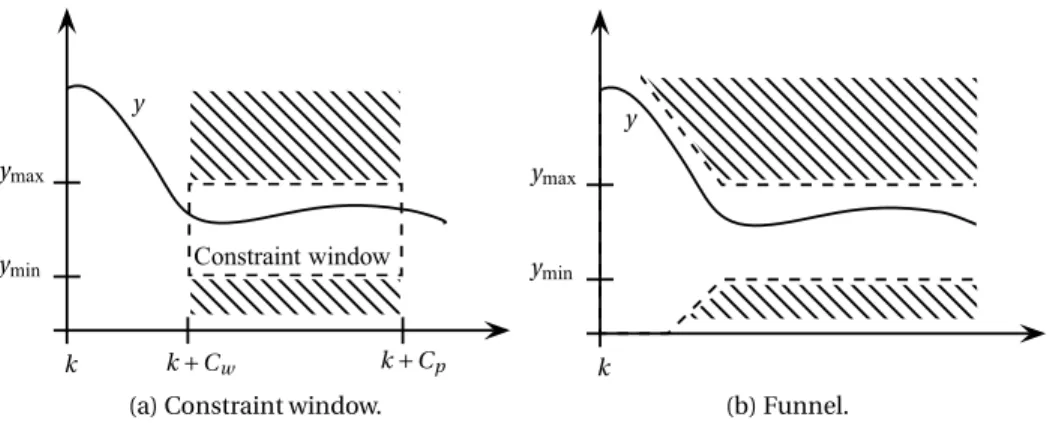
Soft constraints can be exceeded, but it is preferable that the constrained variables are within the original feasible region.

I MPLEMENTATION AND SIMULATION OF

MPC designs

The prediction model is the linearized model representing the distillation column and was given in equation (3.17); The future measurements yk must be estimated to be used in the objective function given by equation (6.23). If the state vector is not measured in the plant, it must be estimated by an observer.

The objective function formulation presented in the following section is given in Camacho and Bordons (2004).

MPC DESIGNS 53

From equation (7.7), we can see that the MPC must estimate the current state and future disturbances. The extended model in equation (7.9) can be used to estimate both states and disturbances. L is the gain of the observer and must be chosen so that the error dynamics (Ω−LZ) is stable.

To ensure that the observer's estimates are correct, the observed system must be observable (Chen, 1999).

MPC DESIGNS 55

MPC DESIGNS 57

The optimization problem minimizes the objective function using the input deviations from the optimization variables stepk tom−1+kas at the current time.mis control horizon, which is not necessarily the same as the forecast horizon as assumed in Chapter 6. The last term in the optimization problem (Equation (7.15d)) arises because the use of soft constraints which was introduced in chapter 6. The unknown variables from the model given in equation (7.14) must be estimated in order to obtain a future good. predictions.

MPC Toolbox estimates three different states: the states of the installation, the states of the disturbance model and the states of the measurement noise model, see Figure 7.3.

MPC DESIGNS 59

The decentralized discrete PI controller can be written as (Balchen et al WhereG0andG1 are matrices containing the controller parameters. We want to make a new state space model that can be used by MPC. When the physical inputs (L, RL, S1 and S2 ) are added as measurements and result in indirect feed from the input to the output for the MPC model.

The MPC Toolbox chosen for the implementation of this controller does not support.

MPC DESIGNS 61

Simulation parameters

SIMULATION PARAMETERS 63

SIMULATIONS 65

Simulations

SIMULATIONS 67

They gave very similar responses, and therefore responses from only one of the MPCs are plotted in Figure 7.8. The simulation is similar to that shown in Figure 5.4, where the effects of steam bypass were tested in closed loop with decentralized control.

SENSITIVITY OF MODEL ERRORS 69

Sensitivity of model errors

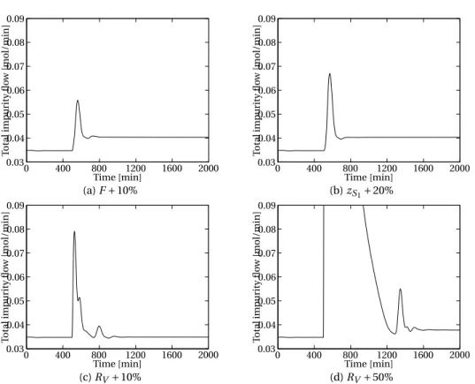
The optimum temperature set points used to control the distillation column were found by minimizing the total impurity flow. 7.24). If we integrate this impurity flux over a simulation and divide by the length of simulationTsim, the average impurity flux for the simulation can be found. 7.25) Therefore, if the average impurity current is large, the control performance is poor. It is not possible to specify a maximum limit for the impurity flow because it depends on how the product purities are specified for the plant in question.

Using these specifications gives a corresponding impurity flow of 0.0425 mol/min, which is probably too stringent a performance criteria since the average impurity flow after a disturbance simulation is more than in nominal operation.

SENSITIVITY OF MODEL ERRORS 71

Thus, the largest changes in impurity flow are due to changes in reflux and liquid splitting. Gain errors at side current inputs do not seem to affect impurity to the same extent. With a decentralized controller, it can be seen that it is important to keep the uncertainty in the fluid distribution low, since it is this input that causes the largest change in impurity flux (see Figure 7.10 and Table 7.5).

To make a better illustration of the consequences of uncertainties in the return flow and the liquid distribution, some more simulation tests were performed.

SENSITIVITY OF MODEL ERRORS 73

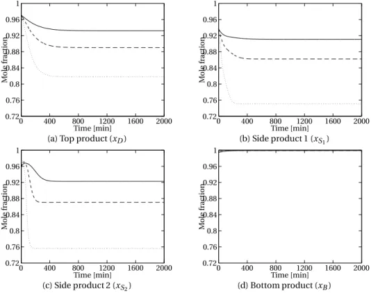
Without considering this, the figures show that the decentralized controller has a generally flatter impurity flux function than the single-layer MPC when the uncertainties are as large as 20%. When the uncertainties were maximum 10%, the single-layer MPC was more robust compared to the decentralized controller according to Figure 7.10.

SENSITIVITY OF MODEL ERRORS 75

Robust performance was also tested for different values ​​of the steam bypass factor presented in Chapter 5. The Kaibel column model was simulated using different values ​​of this bypass factor ranging from 0.010 to 0.100. As explained in Chapter 5, the increased steam bypass compensates for the increased return flow with the controller.

The controllers have a reflux flow saturation of 3mol/min, which gives very poor performance if the bypass factor is too high (above 0.1).

E VALUATION OF ALTERNATIVE MPC

APPROACHES

• Optimization objectives
• Control of product compositions
• OTHER MPC DESIGNS 79
• Other MPC designs

It is possible to have the MPC calculate optimal setpoints for the PI controllers using the actual objective function, e.g. Let the impurity flow be denotedJ, then there may be a possible optimization problem in the MPC. There is another common trick to make the plant more linear as seen from the MBK.

It is possible to perform a logarithmic transformation of the measurements to obtain a more linear behavior.

A PPROACH FOR MPC IMPLEMENTATION AT THE LABORATORY COLUMN

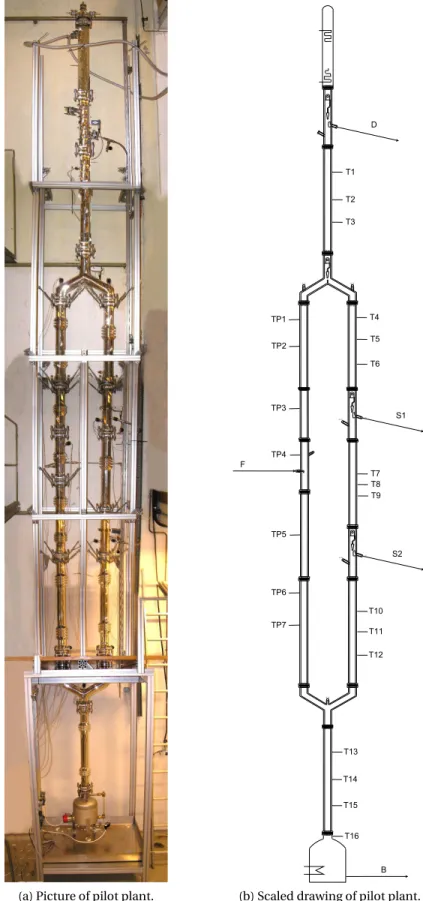
• Laboratory distillation column
• LABORATORY DISTILLATION COLUMN 83
• Model predictive controller
• MODEL PREDICTIVE CONTROLLER 85
• MODEL PREDICTIVE CONTROLLER 87
• Software implementation
• EXPERIMENTS TO BE PERFORMED 89
• Experiments to be performed
• IMPLEMENTATION SUMMARY 91
• Implementation summary

If the forecast model in MPC is based on a parameterized version of the simulation model, the model must be entered. Similarly, estimates for flows can be found at the end of sections 4 and 7 of column;. Two approaches are possible for identifying the forecast model used by the MPC;

The MPC sampling time can be chosen using the same relationship as in the simulation MPC;Ts=Tsettling time.

D ISCUSSION

• Model extension
• MPC simulations
• SIMULATIONS WITH MODEL ERRORS 95
• Simulations with model errors
• OPTIMIZATION OBJECTIVE 97
• Optimization objective
• Implementation at the laboratory column

Without any model errors, the single-layer MPC and the supervisory MPC have almost comparable performance. The supervisory MPC performs slightly better for the large disturbance in the vapor splitting. As we saw in the figures in Chapter 7, the supervisory MPC results in fewer impurity flows when input uncertainties are present, compared to the single-layer MPC.

Supervised MPC also gave better simulation results when time delays were added to the measurements (see Table 7.6) compared to single-layer MPC.

C ONCLUSION

• Concluding remarks
• CONTRIBUTIONS PROVIDED BY THIS THESIS 101
• Contributions provided by this thesis
• Suggestions for further work

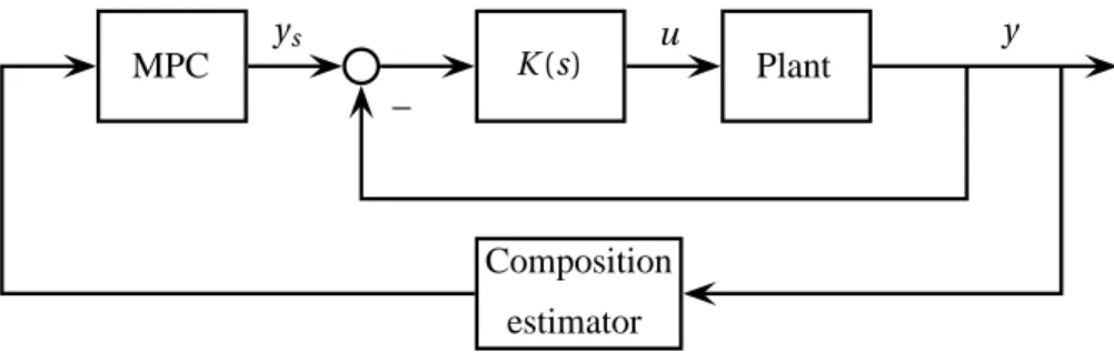
An inferential control structure may be suitable for the control of a Kaibel column, that is, an estimate of its purity, and allows the MPC to optimize these purity estimates. Explicit MPC (EMPC), nonlinear MPC (NMPC), and a quadratic dynamic matrix controller (QDMC) are also discussed as possible approaches for column control. Including physical effects in the simulation model, such as the efficiency parameter, helps to better understand the column dynamics.

A supervisory MPC is found to be the most suitable MPC approach for control of the Kaibel column, both in simulations and for implementation at the laboratory column.

Bibliography

Lecture notes from the course Advanced Control of Industrial Processes, Department of Engineering Cybernetics, NTNU. Industrial application of dividing wall distillation columns and thermally coupled distillation columns. Chemistry Engineer Technik. Chemical Engineering Research and Design/Official Journal of the European Federation of Chemical Engineering: Part A, 75(A6), 539–562.

Dos and don'ts of distillation column control. http://www.nt.ntnu.no/users/skoge/publications/thesis/2009_strandberg/.

Appendix A

Derivation of PI-control matrices

Replacing t with kT from the time domain representation and inserting the integral terms creates the discrete PI controller;. Therefore, for a multi-input, multi-output PI controller, the matrices G0 and G1 in equation (A.1) would be.

Appendix B

Gain error simulation table