Por exemplo, um modelo simples de veículo pode ser facilmente implementado num LTS para estimar o consumo de energia de veículos de competição. Palavras-chave: Competição automotiva, Consumo de energia, Quase-estático, Modelo de 1 roda, Simulação.
List of Tables
List of Symbols
Introduction
State of the art
- Theoretical Overview of Lap Time Simulators
- Energy Consumption of Electric Vehicles
Siegler [1] describes an LTS as a vehicle handling model that connects many different maneuvers, all performed at the vehicle's limit. For a road vehicle, this corresponds to an equilibrium between the wheels and the road at the tire contact patch and a total resistance to the vehicle's motion [9].

Objectives
Cauwer constructed three models, also based on equation (1.4), using real data that could be fitted by linear regression. The third model should be used with real data of all kinematic parameters of the energy consumption equation.
Thesis Outline
The first model took as inputs the distance travelled, time of travel and the temperature. Model 3, which had a lower and unsatisfactory value of correlation, predicted that acceleration would be the larger contributor, accounting for 59% of all energy consumption.
Vehicle Dynamics Fundamentals and Terminology
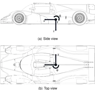
- Axis System
- Cornering
- Tyre Mechanics Terminology
- Slip Angle
- Rolling Resistance
- Camber and Inclination Angle
- Pacejka’s Magic Formula
- Energy Consumption Terms
The slip angle determines the angle between the direction of the tire and the actual direction of its travel. The inclination angle is defined as the angle between the plane of the wheel and the z-axis of the coordinate system in Figure 2.5. The shapes of the Fy(α) and Fx(κ) curves are the same and are usually of the form shown in Figure 2.9.
All these terms are explained here, except for the rolling resistance term which is explained in section 2.3.2. Because the resultant of the car's weight on the tires decreases on hill climbs, the rolling resistance force will also decrease.
Implemented Simulations
Point-Mass Vehicle Model
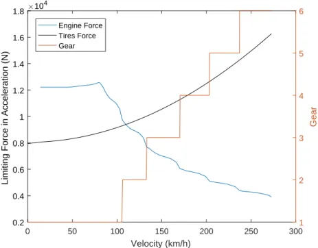
The friction coefficients can be estimated using equations (3.3) of the PacejkaMagic Formula Tire Model using only 5 out of 89 coefficients of the complete model -Pacejka 2002. When the engine is considered, the longitudinal force ( Fx) no longer only limited by the tires because the engine can be the limiting factor. The model of the drive system will be the same for all models in this work and consists of the engine torque curve, as can be seen in Figure 3.2, the gear ratios of the gearbox and the final reduction at the differential.
The driving force produced by an engine is a function of the power produced, which is then a function of the torque, so the engine's limit depends on where in the engine curves the vehicle is operating. In order to achieve this, it is assumed that the selected gear is the one that causes the engine to produce more power for a given linear vehicle speed, thus producing the most driving force out of the entire set of gears.

Simulation Types
- Steady State
- Quasi Steady State
The reverse simulation does the same thing, but in the opposite direction of the track, with the forces moving the car being the braking force of the tires, the drag force and the rolling resistance of the tire, all in the same direction. The final speed profile of the car on a given track is the minimum of the two simulations (forward and reverse) in each segment, as shown in Figure 3.6. The flowchart of the function that implements this iteration in PMSim is shown in Figure 3.8.
In this phase, the calculations start from the same point as the Forward simulation, but go in the opposite direction of the track, as mentioned above. Since it is not at the limit of the tire's capacity, it means that the entry speed of that segment is not the maximum speed and so the tire can still generate a certain amount of longitudinal force to allow the car to reach the maximum cornering speed.
RaceLap Simulator
- Parametrization of a Vehicle in RaceLap
The saturation at the top, for positiveax, is a consequence of the fact that the propulsive force of the engine is the limiting factor, i.e. Also in the chassis configuration there is the vertical position of the vehicle's center of gravity and the moments of inertia along the three ( x, y and z) axes. For the front suspension, these parameters are mapped as a function of the vertical travel of the center of the wheel and the position of the steering rack.
In the rear, the same parameters are needed, but only in function of the vertical movement of the steering wheel. The longitudinal force is given as a function of vertical load and the lateral force is mapped as a function of vertical load and slip angle.
Point-Mass Simulator Choices
Simulation type: Steady State vs Quasi Steady State
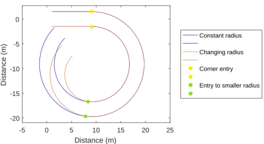
Again, with the ability to simulate both lateral and longitudinal accelerations during cornering, the speed can change and, in this case, decrease to the maximum value it can reach at the smaller radius. This analysis shows how quasi-steady-state is more realistic and therefore more complete than a simple or pure steady-state approach. The two types have the same result if it is possible to describe a corner with the maximum cornering speed, because the lateral acceleration will be maximum: the steady state.
Both steady state and quasi-steady state assume that each segment is an apex (the point on the curve where the vehicle is steady state), but there can be no discontinuity in the speed profile. For this reason, in the rest of this work, the type of simulation used will be quasi-steady state.
Track Model
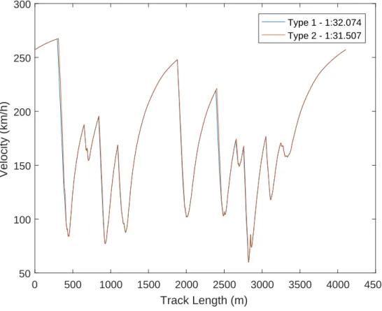
This is possible due to the torque limitation of the motor which creates saturation in the g-g diagrams. There is no saturation in the negative part of the diagrams, so the lower half follows the ellipse equation (3.12). The output of the two track models varies throughout the circuit because the back simulations – see Section 3.2.1 – representing the braking rates will differ.
Since there is no saturation in the g-g diagram in the braking phase, the resulting load is not always the same as when a is zero. Observable in Figure 4.5 is also the confirmation that the difference in the speed profiles is only visible in the braking phases of the lap.
Tyres
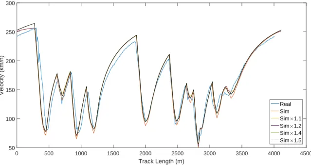
In each of the equations (4.5), the first and second terms correspond to the static and dynamic weight distributions, respectively. Comparison between the single weighted average tire and the two weight transfer tires is made through the resulting speed profiles in one lap of the Estoril circuit in Figure 4.6. It is noted that the differences are mainly on the braking steps, where the weight transfer model results in earlier braking points and thus a lower lap time.
The lap times obtained have a 0.46% difference compared to the actual lap recorded in testing. With this in mind, the single tire method can be used to simplify the code.

Results
RaceLap
- Front Grip Factor
- Final Results
Each tire model provided by the manufacturer is divided into categories corresponding to the tire's grip level, called compounds or treads. All results shown are given identical appex speeds, with the main difference being the speed ramp just before the finish line. This peculiarity of the French circuit makes it ideal to assess the impact of the two grip factors on straight-line behavior.
Taking the RaceLap average of 46.59 m/s, the extra 100 meters means an extra 2.146 seconds, yielding a predicted lap time of 1:37.442 for the same trajectory completed in the best lap of the real test. Since this energy actually comes from the internal combustion engine, this value has to be divided by the efficiency of the powertrain (tank to wheel), which is far from the values of electric vehicles, which approach 100%.
Point-Mass
- PMSim Demonstration
- Final Results
Carrying out the same analysis for the 24 Hours of Le Mans, La Sarthe circuit, the GUI with the corresponding final results is shown in Figure 5.8. The corner names can be identified in the velocity profile and correspond to the circuit map in Figure 5.9. Note that there is no real test data for this track to compare the results to.
Even with the extra 100 meters in the simulation track, the lap time is still significantly lower than the real case. PMSim's lower lap time is a consequence of higher top speeds in the straight and a significant difference in corner speeds in turns 2, 8, 11 and the entry of 13 (see Figure 5.7), just like in the final RaceLap results.

Point-Mass Sensitivity Analysis
- Drag Force (F D )
- Longitudinal Acceleration (a x )
- Downforce (F z )
- Lateral Acceleration (a y )
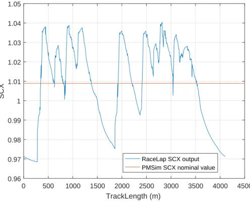
Figure 5.13 shows the change in drag force (FD) in a RaceLap for one lap. The results of the lap time analysis in Figure 5.14 allow a linear relationship between the two variables. According to Figure 5.12, the maximum SCX variation in RaceLap is 0.07, we conclude that the nominal value used in the Point-Mass model is not the cause of the simulation error at maximum speed.
The range for the sensitivity analysis of SCZ values is based on the results of Figure 5.20 and references. These results show that µy is a very sensitive parameter and together with the analysis of Figure 5.23 it is concluded that it is largely responsible for the larger error of the Point-Mass simulation.
Estimator Sensitivity Analysis
- Linear Inertia
- Aerodynamic Drag
- Rolling Resistance
The sensitivity analysis to the aerodynamic term of the energy consumption equation is done in SCX in the estimator, applying a multiplication factor in equation (5.4). The range corresponds to approximately 40% to 180% of the nominal value used in the Point-Mass model. The results are presented as a percentage of the nominal energy consumption result in both simulations: 5.62 kWh for RaceLap and 6.62 kWh for PMSim.
The analysis is done in terms of the fraction of the nominal values of sections 5.1 and 5.2. The results show that the RaceLap results are more sensitive to the estimation of energy consumption as a function of rolling resistance with a slope of 0.0230 energy variation / frr variation.

Conclusions
Achievements
An energy consumption estimator has been successfully implemented in two different lap time simulators with very different vehicle model complexities and thus the outcome of this work can be applied in the design of the energy storage system of an electric competition vehicle. Compared to the actual test lap, the final results of the Point-Mass model are a -6.9% error for lap time, 4.1% error in top speed and an estimation error of 19.56% for energy consumption. This shows that the Point-Mass model is a valid alternative to make vehicle dynamics simulation when only basic vehicle parameters are known and that energy consumption estimation can be made in Lap Time Simulation.
Future Work
Bibliography